(Last revised 1 Jan 2013 - ed.)
Dr. Gary Loechelt has written several monographs on the RATE group’s investigation of the retention of helium in zircons (covered in several publications referenced below, but Chapter 2 (Humphreys, 2005) of the second RATE book is the most complete reference). In May 2010 he was invited to join a discussion of the subject at the Evolution and Origins forum of the Talk Rational discussion board. The discussion included one young-earth creationist (YEC) and several non-YECs with various backgrounds and beliefs.
During the discussion Dr. Loechelt expanded on and explained several of the major issues with the RATE group’s studies. We believe that a small portion of the thread is worth preserving in an easily-accessible form. Herein we present the best messages from that discussion, all written by Dr. Loechelt except where noted. They are not presented in order of appearance. We have performed minimal editing and typo corrections. Links to the original post are at the beginning of each post.
(From this post - ed.) Where did the RATE study go wrong? The key is that if you are going to approximate a multi-domain diffusion system by a more simple single-domain model, you have to focus on the high-temperature part of the Arrhenius curve. In the RATE study, they incorrectly focused on the low-temperature part of the Arrhenius curve. (See for instance Humphreys (2005) pp. 41-45.) The justification for extrapolating from the high-temperature part of the Arrhenius curve down to the temperature of interest can be found in the seminal work by Fechtig and Kalbitzer:
…it is, therefore, allowed to extrapolate the straightline which represents the volume diffusion down to the temperatures investigators are most interested in. (Fechtig &Kalbitzer, 1966)
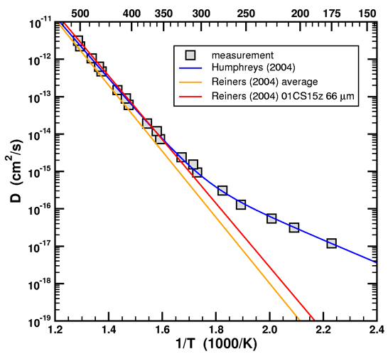
This insight opens up an entirely new possibility to our discussion. We can avoid the issue Humphreys has with Loechelt altogether by repeating the Fenton Hill analysis using diffusion data from another source, such as Reiners, et al. (2004). A single-domain diffusion model should be adequate as long as the kinetic parameters are extracted from the high-temperature part of the Arrhenius curve. For starters, let’s compare the diffusion data between Humphreys (2005) and Reiners, et al. (2004).
Figure 1. Arrhenius plot of data and fitted curve from Humphreys (2005) with single-domain straight-line fits of data from Reiners, et al. (2004).
In addition to the Arrhenius curve given by the average activation energy and diffusion prefactor, I have also plotted the Arrhenius curve extracted from sample 01CS15z 66 µm (Wallowa Mountains). This particular sample happened to have the best match to the Fenton Hill data. Note that in their experiments, Reiners et al. never took their samples below 300C. (The lines on the graph are just exponential fits to the data. To see the actual temperature steps, refer to table 1 of their paper.) I would like to know why Humphreys and his RATE colleagues insisted on having diffusion data at lower temperatures when his own experts never did so in their own publications.
In any event, the diffusion simulations can be repeated for the Fenton Hill zircons using the kinetic data from Reiners, et al. (2004) and the same geometry, boundary conditions, and thermal history. The results are shown below.
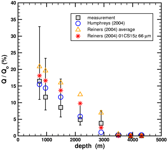
Figure 2. Helium retention ratios versus geothermal well depth from diffusion simulations using the data from Humphreys (2005) and Reiners, et al. (2004).
The Humphreys (2004) data were calculated using a multi-domain diffusion model based upon the RATE diffusion experiment, and the Reiners et al. (2004) data were calculated using a single-domain diffusion model based upon the literature. Note that the diffusion simulations are robust in the sense that small changes in the diffusion kinetics do not drastically affect the outcome. The bottom line is that good agreement to the measured helium retention of Gentry is obtained for both experimental sources for the diffusion parameters, provided that the high-temperature data is used to extract the single-domain diffusion model. If one insists that the low-temperature data be included, as Humphreys did, then a multi-domain diffusion model must be used instead.
Let's now consider the implications of these results on our resident YEC’s argument. His stand is that regardless of the other errors found in Humphrey's work, my work must be rejected because of this statement by Humphreys.
Loechelt is right in claim (A), but wrong in claim (B). He overlooked part of one of his own quotes, in which an expert pointed out that loose helium would only affect the initial steps of the laboratory measurement, because after the initial steps the loose helium would be gone. That is one reason diffusion experts recommend ignoring the initial steps. Our experimenter recommended that, and that is exactly what we did. Thus he felt free to tell us that the rates he measured were accurate depictions of the leakiness for the other 98% of the helium. Ironically, our expert is one of those that Loechelt cites in his section about this issue. Loechelt either completely misunderstood the experts, or he deliberately distorted their meaning. (Humphreys, 2008)
Regardless of whether one considers this statement by Humphreys to be right or wrong, this latest result renders it completely irrelevant. Humphreys cannot make any claim regarding my inappropriate use of a multi-domain diffusion model, because I have replicated the results of my original old-earth model with a simpler single-domain diffusion model. This model relies on the high-temperature steps of a diffusion experiment, and therefore makes no claims about the retention of loosely bound helium. Furthermore, regardless of what Humphreys’ expert told him about the interpretation of his own experiment, that too is irrelevant, because I have now abandoned his work for a better dataset published in a credible academic journal by one of his own experts. And since Humphreys is no expert in the field of thermochronometry, he has no grounds to claim that I misinterpreted another person's work. I merely read the paper and used its results in my calculations. Humphreys’ objections are therefore rendered irrelevant. Are there any counter-arguments to this case? [Resident YEC], what are you thoughts?
(From this post - ed.)
Originally Posted by Resident YEC
OK… Dr. Loechelt… please explain something to me… Dr. Humphreys says you overlooked part of one of your own quotes. Which part of which quote does he think you overlooked and what is he talking about and what is your response to his criticism? Put it in laymanspeak please…
If that is indeed the quote that Humphreys is referring to, then I would argue that he is the one who is misquoting Reiners. I emphasize the parts of Humphreys’ statement that I take issue with.
Loechelt is right in claim (A), but wrong in claim (B). He overlooked part of one of his own quotes, in which an expert pointed out that loose helium would only affect the initial steps of the laboratory measurement, because after the initial steps the loose helium would be gone. (Humphreys, 2008)
First, the use of the word only implies exclusivity. Reiners never makes an exclusive statement. He only mentions the behavior he observed in the initial heating ramp. There is nothing in his statement or experiment to preclude the possibility of helium remaining after the initial ramp. It was just a topic that was outside of the scope of this particular study.
Second, the statement about the loose helium being gone after the initial ramp are not in the quote by Reiners! Humphreys is injecting his own ideas into the words of others. You can draw your own conclusions.
(From this post - ed.)
Originally posted by Poster 5
Why do we see that [diffusion from the low-retentivity domain – ed.] in the lab, but it is not representative of the environment?
In the environment the low-retentivity diffusion domain is in equilibrium with the helium background in the surrounding minerals and rocks. Therefore, there is no net diffusion of the loosely-bound helium either in or out of the sample. In the laboratory experiment, that background is removed before the sample is placed in a vacuum. My model can account for the low-temperature laboratory diffusion data with a helium background anywhere in the range of 0.1% to 10%. The background concentration is not well constrained by the data, but a sensitivity analysis shows that the results do not significantly change over that range, and that all observables can be matched by the model. I can put together a more formal presentation if you wish. Just let me know.
(from this post – ed.)
Originally posted by Poster 5
Oh that is fine thanks, no need for too much more detail! On
what sort of time scales would you expect equilibrium to be reached between the local rock environment and the loose binding areas of the zircons?
It depends upon temperature of course, but 500 to 5000 years is a good estimate which brackets most of the Fenton Hill samples
Originally posted by Poster 5
Also how far away from equilibrium is the tightly bound helium?
Please see the following graph from Loechelt (2008).
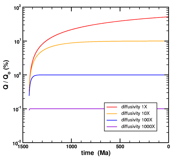
Figure 3. Simulation of the simultaneous generation and diffusion of helium. A constant source function normalized to unity over a time of 1440 Ma was used in a 20 μm spherical model. The diffusivity for each curve is expressed as a multiple of the threshold value for steady-state behavior. The time convention uses zero for the present age and positive numbers for time before present.
It shows the time it takes to approach steady-state in terms of a characteristic diffusivity, which is only a function of time and geometry. For my Fenton Hill model, I calculate that diffusivity to be 5.87·10-24 cm2/s (equation 79). If the diffusivity is lower, then steady-state will not be reached even in 1.5 billion years.
(From this post - ed.)
Originally posted by Resident YEC
So what is the most important issue? My understanding is that it is the “leakiness of helium in zircons.” Just how leaky is helium in zircons? That seems to be a good layman's way of framing the most important question. I had assumed that the answer was “very leaky” but I'm willing to consider your reasons for why you think this is not so. Be patient though… it may take me some time.
True, the “leakiness of helium in zircons” is the central issue. The physical sciences are a quantitative endeavor, which is why they involve so much math. Let me use heat as an example. You can talk about things being “hot” or “cold” and have an intutive idea of what that means. A scientist, however, will want to quantify it and give it a number, called temperature in this case, which can be measured with a thermometer. When you talk about quantifying “leakiness”, the quantity of interest is called diffusivity. Unfortunately, there is no such thing as a diffusometer. How then does one measure leakiness?
One idea would be to measure something that leaks. Put the sample in a vacuum, heat it up, and detect whatever comes out. That is the essence of a diffusion experiment. However, the case of helium diffusion in zircon poses a practical problem. We both agree that the earth must be at least 6,000 years old, right? However, to do an exhaustive diffusion experiment of helium in zircon, one would have to put the sample in the diffusion detector at the temperature of interest for ∼6,000 years (minimum) and wait. No one is going to do this experiment.
What is the solution? Use statistics. In this case, it is the branch of physics called statistical mechanics, which deals with how heat affects things at the atomic level. If you put the sample in a chamber and heat it over various temperature, you can potentially extract a lot of information. In the case of the RATE diffusion experiment, if you look at the gas emitted in the temperature range of the rocks in the ground (i.e. below 250 C), you will find that it amounted to only a few parts-per-million of the total amount of helium present in the sample. What does that tell you about the diffusivity or "leakiness" of the rest of the helium? Very little, actually. Even though the temperature is in the range of interest, the statistical sample size of a few parts-per-million is too small to be an accurate indication of the leakiness of the other 99.999% of gas remaining in the sample. However, if you take the sample up to higher temperatures, you can get the helium to leak out faster, about 26% of the total amount in the case of the RATE experiment. With a sample size of 26%, you can now make a better statistical prediction of the leakiness of the remaining 74% of helium in the sample. The problem now is that you accurately know the diffusivity or leakiness at a temperature that is higher than the temperature of interest.
Statistical mechanics tells us that if the diffusion mechanism is simple, then you can extrapolate the result to a lower temperature by looking at the straight line on an Arrhenius plot, which is a graph of the log of the diffusivity versus the inverse of the temperature. (I know it may sounds strange to you, but the science behind it is very sound.) Here is the Arrhenius plot from the RATE experiment.
Figure 4. Arrhenius plot of data and fitted curve from Humphreys (2005) with single-domain straight-line fits of data from Reiners, et al. (2004).
Notice that the straight line extrapolation of the high temperature data, which represents the leakiness of 99.999% of the helium in the sample, falls well below the low temperature data, which represents the leakiness of only 0.001% of the helium in the sample. The statistics of the experiment say that you should put more weight into the extrapolated leakiness of the majority, and not the leakiness of the minority. Farley, Reiners, and company (whom Humphreys considers to be experts) determine the diffusivity by extrapolating from the high temperature data. Humphreys and company relied only on the low temperature data. Here is where their error lies. If you don't believe that Farley and company ignore the low temperature data, then consider why Reiners, in his 2004 paper, never even bothered to take his samples below 300 C!
(From A Response to the RATE Team Regarding Helium Diffusion in Zircon, Loechelt, 2009 - ed.)
Humphreys made this claim apparently without performing any calculations. In contrast, I had previously performed these calculations. In Appendix C of my technical paper (Loechelt, 2008), I discussed how the kinetic parameters of my multidomain diffusion model were extracted by performing forward modeling of the stepwise heating diffusion experiment inside a nonlinear optimization loop. Although not shown in that paper, this extraction technique required the explicit calculation of the fraction of gas released during the diffusion experiment by both the high-retentivity and low-retentivity helium domains. The results of these calculations are shown shown in Figure 4 below, using helium diffusion data from the 2004 RATE CRSQ paper (Humphreys et al., 2004).
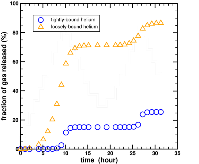
Figure 5. Calculated fraction of helium gas released during a stepwise heating experiment for a two-domain diffusion model using the heating data from Humphreys et al., 2004.
As can be seen, 30% of the loosely-bound helium (orange triangles) survived the first heating ramp at 15 hours, and 15% even survived the second heating ramp at 30 hours. Therefore, enough loosely-bound helium remained to explain the low-temperature diffusivity through-out the entire experiment. Although the exact gas release values at any given time step are sensitive to the assumptions used in constructing the multidomain model, most notably the partitioning fraction between the two helium domains, it does demonstrate that it is possible for a fraction of the loosely-bound helium to remain throughout the entire experiment, contrary to Humphreys’ unsubstantiated claims. (Loechelt, 2009)
(Adding the temperature step information to the figure may clarify the situation. Note that very little helium is released when the temperature is decreased, or even when the temperature is increased following a decrease. From this post - ed.)
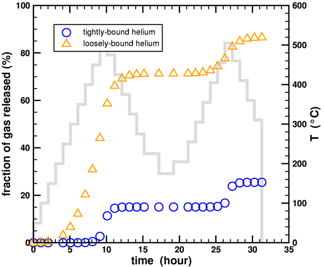
Figure 6. Calculated fraction of helium gas released during a stepwise heating experiment for a two-domain diffusion model using the heating data from Humphreys et al., 2004, with the temperature history of the experiment superposed in light blue (scale on right side).
The temperatures are not a linear ramp but a stair step. I have captured this effect in the plot.
(From this post - ed.) From Poster 2:
The neglected domains are negligible when calculating helium release in the wild based on a previously developed model of diffusion rate as a function of temperature. The neglected domains are not negligible when developing a model of diffusion rate as a function of temperature and using data measured at temperatures low enough for releases from the two domains to be comparable, without accounting for the presence of two domains.
At the “low” temperature (about 1000/T > 1.8 in Figure 1 above) the amount of helium released from the “loosely bound” domain is comparable to the amount of helium released from the “tightly bound” domain. The data points bending over to the right are in a sense artifacts, because they do not represent what would be measured if we could measure over long periods at realistic pressures in the wild. (At least that's my understanding). If we could measure in the wild, we would see the points continuing along the red and yellow lines.
Dr. Loechelt developed the yellow line from data from Reiners, et al. (2004), using a single-domain model and only data from temperatures > 300C where the release was predominantly from the “tightly bound” domain. Reiners didn't do any measurements below 300C. Loechelt has also used Humphreys’ data to derive a similar line (not graphed anywhere as far as I know) from all of Humphreys’ data using a model that accounts for the presence of the two domains.
(From this post - ed.)
Originally posted by Poster 4
The more that Humphreys paper is investigated the worse it
becomes. How can you have a “knee” in your model if you're using a
single-domain (i.e. single diffusion coefficient)?
Let me try to clear this up for you. First, let's start with what was actually measured.
In principle these two measurements can be related to one another by applying a suitable diffusion model. The required elements of such a model are
The idea behind the RATE study was to compare both a young-earth and old-earth model as a test for the age of the earth. In principle, it is not a bad idea provided you do the modeling correctly. As I have already documented, the RATE team made major mistakes in all four items above. Never-the-less, they proceeded with the comparison.
There are actually two different approaches you can take in comparing the models [to measured data – ed.]. My approach is called a forward modeling method. I take all four items above as inputs, and the model calculates the retained fraction of helium which I then compare to the measured data of Gentry. In this approach, I like displaying my final result using graphs like this
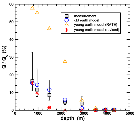
Figure 7. Simulated and measured helium retention ratios versus geothermal well depth. Two young-earth models (triangles and stars) and one old-earth model (circles) are considered. Measured data (squares) are from Table 1 in Loechelt (2008).
Humphreys used a different approach called inverse modeling. He took items #1, #2, and #4 as inputs along with the measured helium retention data of Gentry. This left item #3, the helium diffusivity, as the remaining unknown. Given these inputs, the inverse modeling method allowed Humphreys to calculate the diffusivity that would have been required to replicate the measured helium retention fraction. He then compared that number to the independently measured helium diffusivity of the laboratory experiment. Accordingly, Humphreys likes displaying his final result using graphs like this
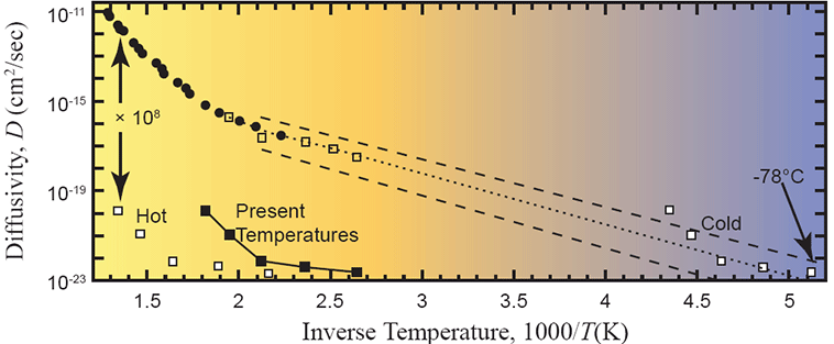
Figure 8. Arrhenius plot of measured data with the defect-line domain extrapolated (dotted line) and several “uniformitarian models” overlaid (white and black squares). From Humphreys (2005).
In principle, both forward and inverse modeling methods should work. In practice, using the inverse modeling method is a bad idea. This is yet another poor decision made by Humphreys and his team. Here is the problem. Humphreys’ inverse modeling approach only works if
The reasons are obvious. If you have multiple diffusion domains, how can you determine two numbers from only one equation? Similarly, if the temperature varies, then so does the diffusivity. Where then do you plot the result on the Arrhenius curve to compare with measured data? My forward modeling method can handle diffusion domains and temperature histories of arbitrary complexity. In the end, I still only have to compare my result to a single measured helium retention fraction.
Getting back to your original question now, since Humphreys’ inverse modeling method treats the diffusivity as an empirical output, it can have any shape depending on the inputs you feed into it. However, the interpretation of the result is inconsistent, as you pointed out. If the output does not lie along a straight line, then one would have to question the starting assumption of a single diffusion domain. Humphreys never did.
(from this post – ed.) I have created an annotated version of this figure to facilitate my discussion.
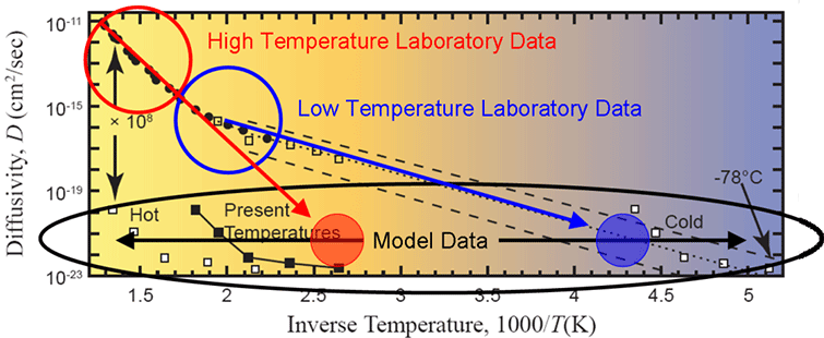
Figure 9. Arrhenius plot of measured data with the defect-line domain extrapolated (dotted line), several “uniformitarian models” overlaid (white and black squares), and several regions identified (see text). Modified from Humphreys (2005).
The figure is an Arrhenius plot of helium diffusivity versus inverse temperature. Consider the following two datasets on this plot. First, there is the diffusivity that was determined by a direct laboratory measurement. This dataset is labeled as such on the graph. It has a characteristic form in which the diffusivity increases with higher temperature (i.e. lower inverse temperature). If the diffusion was by means of a simple kinetic mechanism, theory predicts that all the data should lie along a straight line. In fact, it does not. The data has a distinct kink around 300C (1000/T = 1.8). This kink implies that more than one kinetic mechanism is at work. Since the shape of the curve can be well described by two lines, a two-component mechanism is inferred. I have circled the two components as a high temperature regime and a low temperature regime.
The second dataset is a model diffusivity. The model diffusivity was determined by Humphreys’ inverse modeling approach in which he inverted the model equation for his uniformitarian model (equation 16) and solved for diffusivity. The parameters in the uniformitarian model equation are the helium retention fraction (Q/Q0), the domain radius (a), the diffusivity (D), and the time (t). Notice that temperature does not enter into the model equation. Humphreys used the data from Gentry to set Q/Q0, 30 µm for a, 1.5 billion years for t, and solved the equation for D. Depending on the sample, the value for D ranged from 1·10-20 to 1·10-23 cm2/s. Despite Humphreys’ multiple mistakes, this estimate is actually reasonable.
Now the task is to compare the two diffusivities on the Arrhenius curve. However, there are two fundamental problems. First, the model dataset has no temperature. The model sets its vertical position on the y-axis but provides no constraint for its placement on the x-axis. I depict this fact with the black horizontal arrows spanning the width of the plot. Humphreys had to use some heuristic argument to set the temperature. You can see different choices for his temperature by his “sliding” the dataset both left (hot) and right (cold) from the present temperatures.
The second fundamental problem is that the diffusivity measured in the laboratory did not extend down to 1·10-20 cm2/s. The reason for this limitation is simple. The helium leakage rates are too slow at this diffusivity to have any measurable signal in any reasonable length of laboratory time. Because of this limitation, the laboratory data has to be extrapolated down to lower diffusivities in order to make a comparison to the model. Humphreys extrapolated the low-temperature data (blue line) to the level of the model diffusivity (filled blue circle), and concluded that subzero temperatures would be required to make the uniformitarian model work. Since this was clearly impossible, he argued, an old-earth interpretation can be rejected.
However, Humphreys failed to discuss a second possibility. The high-temperature laboratory data (red line) can also be extrapolated to the level of the model diffusivity (filled red circle). If this is done, it intersects the model diffusivity at reasonable temperatures which are representative of where geologic data indicates that these samples spent most of their time over the last 800 million years. This is the uniformitarian interpretation that Humphreys should have addressed, but conveniently chose to ignore. Like most young-earth arguments, uninformed people can be swayed by them if they don’t know enough to ask the right questions. We have enough information to ask these kinds of questions now.
Why did Humphreys extrapolate from the low-temperature laboratory data instead of the high-temperature laboratory data?
Since his writings do not address this question, let's search the relevant scientific literature for clues.
…it is, therefore, allowed to extrapolate the straightline which represents the volume diffusion down to the temperatures investigators are most interested in.
If you read the context of this statement and the preceding case studies, it is clear that by “volume diffusion”, they are referring to the high-temperature (not low-temperature) portion of the laboratory data.
2. The RATE experiment was performed by Reiners and his associates. Consider the fact that in his published work on helium diffusion in zircon, he did not take his samples below 300C. He explicitly chose to work with only high-temperature laboratory data.
Given the precedents against Humphreys’ interpretation of the laboratory data, I would like to hear an explanation as to why an extrapolation of the low-temperature laboratory data is valid.
(From this post - ed.) Yes Poster 3, I think your synopsis is better than what I was planning to write. (I am too wordy at times.) Basically, there are more right ways to model the data than wrong ways. Humphreys and company just happened to do it wrong.
Right Ways
Wrong Way
3. Use a single-domain model and extract the diffusion parameters from the low-temperature data.
You are also correct that the cut-off temperature cannot be exactly known in advance. In principle, there can be variability from sample to sample. Having said this, I think it is more than coincidence that in Reiners (2004), they never bothered taking the temperature below 300C, and in Humphreys (2004), the cut-off is right around 300C. Coincidence or experience?
Speaking of experience, I find these series of quotes by Humphreys interesting.
The Nevada zircon data did not extend to low enough temperatures to compare them with the He Retentions. (Humphreys, 2005)
The “Nevada zircon data” refers to Reiners (2002). Humphreys is complaining that his diffusion experts did not take the temperature below 300 C.
After that, in the summer and fall of 2002, we tried several times to get lower-temperature zircon data. (Humphreys, 2005)
Humphreys was not satisfied that the original helium diffusion experiment performed by his experts only went down to 300C.
This time we asked the experimenter (a) not to etch the crystals in HF (unnecessary anyhow because no sieving was needed) and (b) to get zircon diffusivities at lower temperatures. (Humphreys, 2005)
Three times Humphreys insists on going to lower temperatures. Notice it is the amateurs telling the experts what to do, not the other way around. I wonder what his diffusion experts thought? But they were under contract, and as the saying goes, the customer is always right. What did they find at lower temperatures? See Figure 1, above. Just below 300C, the Arrhenius curve begins to deviate from a straight line. This is exactly the point at which Fechtig and Kalbitzer advise the users of their diffusion method to ignore the data. (Fechtig & Kalbitzer, 1966). Coincidence? Or did Farley and Reiners know that they were wasting their time (but someone else’s money) by investigating here?
Originally Posted by Poster 3
Since our resident YEC seems somewhat
reluctant to answer my question, perhaps either yourself or Dr Loechelt could
oblige? Is there any a priori justification in Humphreys’ conclusion that all
of the helium released from the crystals would be endogenous?
I think most of the helium was endogenous. The zircon crystal has a high affinity for radioactive elements like uranium and thorium, which usually makes it more radiogenic than its host rock. Most of the helium was probably generated inside the crystal by radioactive decay.
An interesting prediction of my multi-domain diffusion model, however, is that the “loosely-bound” helium could not have survived inside the crystals for 1.5 billion years. Then why was any found in the RATE samples? I believe that the “loosely-bound” helium was exogenous, and that the “tightly-bound” helium was endogenous. All it takes is about 0.3% “loosely-bound” exogenous helium to account for the low temperature tail in the diffusion experiment. This is a very reasonable background helium level for this rock formation, based upon whole rock elemental analysis. That 0.3% “loosely-bound” exogenous helium would be trapped inside the zircons by the host rock until crushed and heated under vacuum in the diffusion experiment. Then it would escape, manifesting itself as a low-temperature tail in the Arrhenius curve. Seeing a small quantity of helium being so quickly released at low temperatures, Humphreys concluded that all the helium must also be so “loosely-bound” in the crystal at low temperatures, and constructed his model accordingly. He totally ignored the temperature dependence of the majority of “tightly-bound” helium that was liberated at high temperatures. Herein lies the fatal error.
[Another point to mention is that any exogenous helium will preferentially occupy defect sites over lattice sites. Just as it is relatively hard to diffuse a helium atom out of a lattice site, it is equally hard to diffuse a helium atom into a lattice site. Any background helium will favor the cracks and defects in the crystal structure. The internally generated helium does not have this restriction. The high-energy helium nuclei that are generated from alpha decay can easily penetrate deep into the crystal lattice – ed.]
(From this post - ed.) Let me make one more attempt at explaining the helium diffusion experiment and how multiple diffusion domains complicate its interpretation. First, in diffusion modeling, an important physical quantity is the particle flux, which represents the number of particles which flow across a unit area per unit time. For a two-domain system, the flux can be represented as
F = -D1 gradient(N1) - D2 gradient(N2)
For the sake of argument, let the subscript 1 represent the high-temperature domain and the subscript 2 represent the low-temperature domain. The problem with interpreting the results of a diffusion experiment when there is more than one diffusion domain is that the concentrations N1 and N2 cannot be determined from the data. The only constraint is imposed by the total helium yield.
N = N1 + N2
Even though D1 and D2 can be measured, the model cannot be uniquely specified without also knowing the respective concentrations. To our resident YEC: this is another way of answering your question. You say that if a vacuum diffusion experiment is valid, then we should trust the diffusion numbers regardless of temperature. I agree with you. However, the issue is not the validity of the diffusion parameters, but the completeness of the experiment. There are more unknowns in the model than the experiment can answer. Therefore, some additional information or theoretical argument must be given to specify the last unknown. This unknown quantity can be represented by the concentration ratio
R = N2 / N1
In my multi-domain diffusion model, I used a ratio of
R = 0.3/99.7
This number was not well constrained by the data. However, I did a couple of sanity checks. First, I ran a sensitivity analysis showing that any ratio between 0.001 and 0.1 gave essentially the same result. This two-order-of-magnitude range showed that at least the model was robust in the limit of a small gas fraction. Second, I checked that ratio against the background helium concentration which would be expected from the whole rock radiogenic element concentration. Third, I checked the literature and found that when a multi-domain diffusion model was used, typically at most a few percent of gas was assigned to the low-retentivity domain.
If it is true that the gas ratio is small, then the inequality
N2 << N1
should hold. This provides the justification for reducing the flux equation to a single domain.
F = -D1 gradient(N1)
Since N2 << N1, the contribution of the second domain to the flux will also be small. This limiting case provides the justification for using only the high-temperature data in the diffusion model. The problem is not that the value for D2 is somehow wrong or bad. It is merely a consequence of the fact that if the second component N2 is small, then it really doesn't matter what the value for D2 is. The flux over time will be dominated by N1.
Now, what did Humphreys do? That is a good question. Here is another point where he failed to adequately document his assumptions in my opinion. I cannot critique his approach without knowing what he did, so I will have to make a few guesses. One possibility is that he assumed
N2 >> N1
Then his analysis would be correct. However, it is hard to justify this case. First, much more gas was released in the high-temperature steps of the experiment than the low-temperature steps. This would imply that
N2 << N1
Furthermore, Humphreys assigns N1 to an intrinsic diffusion mechanism and N2 to a defect diffusion mechanism. I think this is reasonable. If it is true, then there must be more intrinsic atomic sites than defect sites unless the crystals are badly damaged. However, Humphreys published SEM photographs of the crystals showing that the crystalline form was good. Also, Farley reported that the helium content was not so high for radiation damage to be a serious concern. All of these factors would again argue that
N2 << N1
There is another possibility. Perhaps Humphreys made the simplification of
N1 = N2 = N
In that case, the flux equation would simplify to
F = -(D1 + D2) gradient(N)
The extra variable is now eliminated and the diffusion model can be expressed unambiguously, but what does this simplification mean? I have no clue. To me it is completely unphysical. It says that a given helium atom can be in both an intrinsic atomic site and a defect site at the same time! How can one helium atom be in two different places at the same time? I cannot find an answer to these questions in any of Humphreys’ writings, and until a reasonable answer is given, I have to dismiss the helium diffusion in zircon study, especially in light of the contrary evidence found in the published literature.
(From this post - ed.)
Originally posted by Resident YEC
Dance as much as you want. There is absolutely no escaping that Humphreys made a specific, risky prediction right there on p. 348 (Humphreys, 2000) and the lab results confirmed his prediction. Or do you think he paid Farley extra to make the results land squarely on his graph?
Originally Posted by Loechelt
… Why would Humphreys pay Farley extra to fudge the data to fit his model when it was so much easier to fudge the model to fit the data! He had to change the dimensions and boundary conditions of his model otherwise it would not fit the data! I pointed this out over a year ago in my reply to Humphreys (Loechelt, 2009). Please see the following graph.
The red stars show what Humphreys' unfudged model would have looked like. It does not match the measured data at all.
What do you mean “would have looked like”? The red stars represent your “alternative model”, no?
I'm looking at the original prediction (Figure 7 from Humphreys (2000) has been added here for convenience - ed.)
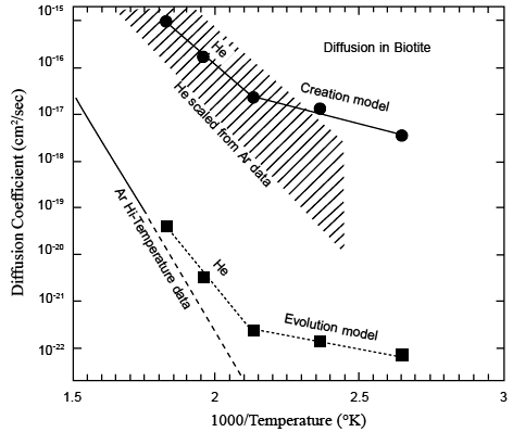
Figure 7 from Humphreys (2000). Predictions of yet-future experiments on He diffusion through biotite, using the observed He retention in Jemez zircons in two very different theoretical models. An evolutionist model (gigayear timescale) predicts the line with square points. A creationist model (kiloyear timescale) predicts the line with round points. The solid line shows experimentally-measured Ar diffusion in biotite [Grove and Harrison, 1996], extrapolated down by the dashed line from high temperatures to these temperatures. Rough extrapolations from those data using He and Ar diffusion observed in other minerals [Carrol, 1991; Lippolt and Weigel, 1988] suggest that the He-in-biotite measurements will fall into the shaded band shown. Thus He diffusion measurements in biotite are likely to reject the evolutionist model and confirm the creationist model.
right now. I see five points corresponding to “the Creation model” they are (best I can tell reading the graph) at the following coordinates:
Those were made in 2000 without any reference to subsequent data. They look like they correspond to the yellow triangles in your graph, identified as “RATE model 2003”.
Why isn't Resident YEC right, then, when he says the 2000 predictions were borne out by the eventual data (the gray boxes)?
Poster 1, you have to go back to the discussion in my reply to Humphreys (Loechelt, 2009). Briefly, the argument goes like this.
Humphreys' Model 2000: Assume Dzircon >> Dbiotite. Then a reasonable geometry is a zircon-sized cavity in a biotite sphere. The radius of this cavity representing the zircon was determined to be 22 μm.
Farley's Measurements 2003: Measurement shows that Dzircon << Dbiotite. Therefore, the diffusion model has to be revised.
Alternate Model: Given the two points above, the simplest and most obvious way to change the model is to turn it “inside-out”, making the cavity a solid sphere and ignoring the biotite. Since Dzircon << Dbiotite does not affect the original choice for the geometry, the radius of the solid sphere should again be 22 μm. This model was used to calculate the red stars. Note that the numbers change from the 2000 model because, when you change a model you usually expect the out-come to be different. Funny how that works in science.
Humphreys' Model 2003: Additional changes were made to the model. Humphreys started by considering a two-material system. However, in the end, he simplified that system so that Dzircon = Dbiotite even though his own data showed that Dzircon << Dbiotite. Furthermore, he increased the radius of the zircon sphere from 22 μm to 30 μm for apparently no good reason. Why all these additional changes, especially the choice of Dzircon = Dbiotite when measurements showed that Dzircon << Dbiotite? This model was used to calculate the yellow triangles.
Farley's Measurements 2003: This data was available before Humphreys published his new model. If one extrapolates the measured diffusivity of helium in zircon down to temperature of interest, one gets the blue line. Three of the yellow triangles lie almost exactly on the blue line. Is this a remarkable and risky prediction? No, it cannot be called a prediction because the new model was published after the measurements were made. Is it pure coincidence? I will let you decide. Did Humphreys make these apparently unphysical changes to his 2003 model so that it would match the blue line? I cannot rule out this possibility. What I can say is that Humphreys used Dzircon = Dbiotite when his own data showed that Dzircon << Dbiotite, and that he changed the size of his zircon from 22 μm to 30 μm. When I follow through with the calculations, I find that it moves the red stars to the yellow triangles, 3 of which just “happen” to lie on the blue line. Again, there is no prediction here since all of this information was known at the time Humphreys published his revised model.
Farley's Measurements 2004: These are the gray squares in the figure, most of which happen to lie along the blue line from the 2003 measurements. Since three of the yellow triangles also lie along the blue line, they also match the gray squares. It is a simple consequence of the mathematical law
If A = B and B = C then A = C (transitive law of equality).
Now Humphreys' publishes his 2003 model and his 2004 measurements on the same plot and declares victory in a remarkable prediction. However, how remarkable is this agreement of the model to the measured data? Two questions need to be answered.
My argument is that in order for the agreement between Humphreys' model and experiment to be considered significant, these particular choices in the model must be defended against all reasonable alternatives. Humphreys has not done this. In contrast, I can make a good case that the alternate model is more physical. In particular, it takes into account Dzircon << Dbiotite. I argue that based upon the known physics, it is a better choice of geometry and boundary conditions. However, it does not agree well with measurement, which suggests that the fundamental flaw in the model is related to its young-earth assumptions.
(from this post – ed.)
Originally Posted by Poster 2
…
I believe he's saying that if you substitute “whichever material is the rate-limiting factor” for “biotite” in Humphreys' RATE I analysis and prediction, then you get a valid prediction that is, in Resident YEC's opinion. borne out by the later measurements. I.e. Humphreys' made a mistake thinking that biotite was the rate-limiting material but that error doesn't really invalidate the overall analysis.
If that were all there was to it, IMHO Resident YEC would have a point worth considering, at least…
Maybe “worth considering” – for a moment, anyway. But I still have trouble – I've been trying to articulate this over several posts now, and I don't think I've succeeded. Let me try one more time.
Assuming we're sticking with this “spherical zircon embedded in biotite” model, if diffusion through zircon is the limiting factor, you have to model the kinetics of travel of helium from every point within the sphere to the surface. It's going to take a lot longer for the He atoms in the center to wend their way to the surface than the ones right at the edge. If biotite is the limiting barrier, the sphere is essentially a homogeneous bubble of helium, and all you need to do is model the rate at which the He in the bubble irreversibly enters the biotite matrix; position of the He within the bubble is immaterial, since all the He atoms will be bouncing around at every point within the bubble gazillions of times before finally entering the biotite matrix. And then the dimensions of the stuff that's supposed to be limiting – the biotite – doesn't enter into it at all.
So it seems to me leaving the mathematics – and the model – the same, but just relabeling the limiting substance from “biotite” to “zircon” just makes no sense at all.
Does anyone understand my point here? Has everyone understood all along, and it's just my imagination I'm not getting it across? Am I wrong?
Poster 2, I will try to answer what I think your question is. The way I look at it is that Humphreys' change in models is rather strange for several reasons. Among the many unanswered questions that advocates of his position fail to answer, the most curious one for me is how can you fundamentally change a diffusion model geometry and boundary conditions without changing the numerical result by more than 0.5%? Humphreys notes this peculiarity but offers no explanation as usual. Also, I conceptually understand his 2000 biotite model but not at the mathematical level. He never published the model equations, and I never bothered to look up the reference. When I came across the RATE 1 book, Humphreys' 2003 ICC conference paper had already been published, so I started immediately with his new model. Also, I created the “alternate model”, so there are actually three models to consider here.
Humphreys' 2000 RATE 1 Model: The key features are a zircon cavity with a dimension of a = 22 μm in a presumably infinite biotite matrix. The only critical parameters are D of the biotite and a of the sphere.
Humphreys' 2005 RATE 2 Model: This model was first published in his 2003 ICC conference paper. The key features are a zircon sphere inside a larger biotite sphere. Although Humphreys' own data shows that the two materials have vastly different diffusivities, he treated them both the same, so for all practical intents and purposes you can treat the problem as diffusion through a homogenous material of diffusivity D looking at how much helium remains inside the inner radius. The critical parameters are D, a, and b (diameter of the biotite sphere). Formally speaking, this model has one extra parameter (read fudge factor) to work with.
My Alternate Diffusion Model: This model takes into account the orders of magnitude difference in diffusivity between zircon and biotite by ignoring the biotite altogether. Although this approximation is not strictly correct, it is much more physically reasonable than treating them equal as in model #2. The geometry of the model is a solid zircon sphere of radius a = 22 μm like in model #1. Likewise, the only critical parameters are D of the zircon and a of the sphere.
Now Resident YEC’s argument is that it does not matter whether the zircon or the biotite is the limiting factor to diffusion -- It is all the same. Mathematically, that means using the same value for D in all three models regardless of whether it is zircon or biotite. I question the reasonableness of doing this on physical grounds. Never-the-less, it is a well-posed problem mathematically.
Now we come to what I think is your underlying question, if I understand it correctly. Suppose we substitute the same value for D in the three models above, would we then expect them all to arrive at the same answer? The answer is a categoric NO! Even with the same diffusivity D, the models have different geometries, hence different mathematical forms, and also different physical dimensions. Quite clearly, models #1 and #3 give entirely different answers, which is no surprise. More surprisingly, models #1 and #2 give essentially the same answer. It is not clear a priori why this would be the case.
If you are really dying to know why, then the only answer is to look up the equation to model #1 and perform a formal mathematical analysis comparing it to model #2, which has its equation published in the RATE 2 book. I am totally capable of doing the analysis. I have not done it because 1) I did not look up the reference. 2) I do not have the time. 3) I am not really that interested. Humphreys' helium in zircon dead horse has already taken a severe beating. Never-the-less, I still like math a lot. Therefore, I will make a deal with you. If you will look up the reference to model #1 for me (Carslaw and Jaeger (1959), pp. 256-257 — see the RATE 1 book for details), I will perform the mathematical analysis. Intuitively, I can see the comparison taking one of two branches. (I assume that numerically models #1 and #2 do agree to within 0.5% or so. Amazingly, I still trust Humphreys to get a few things right.)
Perhaps in a limiting case, the two models are not that different. After all, in model #1 the helium gets a “free ride” for 22 μm and then has to diffuse at a rate of D into an infinite space. In model #2 the helium has to diffuse at a rate of D through at most 30 μm of zircon before diffusing again at a rate of D through 1000 - 30 = 970 μm of biotite. One could argue that since there is 33x the amount of biotite to zircon, the extra zircon does not slow the helium loss by that much. It is primarily the biotite restricting the loss of helium which is opposite the claim which Humphreys makes. Self-consistency was never a strong point for young-earth creationism.
Perhaps the size of the zircon core makes a significant difference mathematically. Then, apparently the combination of a = 22 μm for model #1 and a = 30 μm and b = 1000 μm for model #2 happen to cancel, or at least mostly cancel. If this is indeed the case, then one could reasonably accuse Humphreys of fudging, since the parameter a was changed arbitrarily and the parameter b is not well constrained. (How can one be reasonably sure that all these zircons came from biotite flakes of the same size?)
Basically, I believe those are your two options. The remarkable agreement between models #1 and #2 is either artificial or contrived. I really don't care which one it is, but if you provide the reference, I will do the math!
(from this post – ed.)
I got it (Carslaw & Jaeger on-line second edition - ed.) and tried looking up the equation. Boy, I am really losing confidence in Humphreys' work. It is far worse than I thought, if that could even be possible. When I went to pp. 256-257 of the reference by Carslaw and Jaeger, it was not clear to me how it applied to the problem at hand. Therefore, I double checked my printed copy of the RATE 1 book to make sure that I read the reference correctly. Sure enough, it lists pp. 256-257 as the reference (page 347 of the RATE 1 book (Humphreys, 2000)). Then I had a wild idea. What is the reference in the electronic PDF copy of the RATE 1 book. It is pp. 234-235, not pp. 256-257. No kidding! The page numbers for the reference have changed between the printed and the electronic copies of the book. Does anyone recall a correction statement for the electronic copy?
I thought that maybe Humphreys had just corrected a typo in the printed copy, so I decided to see if there was any indication in the endnotes.
Printed Version: Carslaw, H. S., and J. C. Jaeger, Conduction of Heat in Solids, second edition, Clarendon Press, Oxford, 1959. The solutions apply just as well to diffusion of He as they do to diffusion of heat. Volume-integrate (o to a) eq. (6) on p. 257.
Electronic Version: Carslaw, H. S., and J. C. Jaeger, Conduction of Heat in Solids, second edition, Clarendon Press, Oxford, 1959. The solutions apply just as well to diffusion of He as they do to diffusion of heat. Apply case IV, p. 235, to eq. (8) on p. 234.
So the difference is not just a correction of a typo, but a change in the actual equation and method he used for his calculation. Very interesting. Furthermore, when you go to the reference in the printed version, the section heading reads “the instantaneous point source”. It discusses “the temperature in an infinite solid with initial temperature f(x,y,z) as due to liberation of heat at t = 0 over the volume of the solid”. Ignoring the difference between heat and He diffusion, the remarkable statement is that these equations pertain to “an infinite solid”, not a hollow cavity. It looks like Humphreys did not even use the correct equation from Carslaw and Jaeger in his 2000 model. Printed version, we must add.
But wait, there is more. He used a different equation for his 2000 model. Electronic version, we must add. What do we find on pp. 234-235 of his reference this time? The section heading reads “the sphere 0 < r < a with initial temperature f(r), and surface temperature phi(t)”. In other words, this section does not discuss a hollow cavity either, but a solid sphere. Go figure. Equation (8) on p. 234 is for the average temperature inside the sphere. However, the average temperature is not the same as the temperature inside a cavity of uniform temperature. So not only did Humphreys change his equation from the printed version to the electronic version of the RATE 1 book, he screwed up the equation a second time. No where in either reference from either the printed or electronic version of the book do I find the correct equation for diffusion from a cavity into a surrounding medium.
Young-earth creationism relies upon miracles, and we have just witnessed another one take place. Humphreys made a “specific and risky” prediction in the printed version of the 2000 RATE 1 book, used the wrong equation for his helium filled spherical cavity model, changed the equation he used in the electronic version of the RATE 1 book, used a different wrong equation for his helium filled spherical cavity model, further changed his model again in his 2005 RATE 2 book to be two concentric spheres with identical diffusivities even though they are vastly different materials, claimed that his prediction applied to zircon now instead of biotite, and amazingly got the same numbers he published back in 2000. A miracle has happened!
If that isn't enough for you. Humphreys defends his work in 2008 claiming that experimental data had confirmed his remarkable prediction back in 2000! To top it off, he boasts that
This contrasts starkly with the RATE helium project. It was a multi-author effort, and it had more than seventeen reviewers and editors as it appeared in five technical publications, one of which is non-creationist. (Humphreys, 2008)
So these reviewers and editors did not notice or object to all these erratic changes. Resident YEC, I would like to see how you defend Humphreys in light of these new revelations.
But I know you will. After all, it is a little too harsh to criticize the work of a creation scientist just because he reads graphs backwards, changes the material he uses in predictions after he has the data, uses the wrong equations for his models, changes the contents of electronic documents from their printed originals without any clear notice, and publishes other people's data without their knowledge or permission, because in the end the only thing that matter is that it was published by his peers and supports the conclusion of a young earth.
(from this post – ed.)
Originally posted by Poster 1
Originally posted by Loechelt
There may be some degree of coincidence in a wrong model giving a numerically right answer, but there are also more subtle manipulations that Humphreys could have done as well. For instance, Poster 8 pointed out that the measurement of diffusivity gives D/a2, not D directly. Therefore, in changing a from 22 μm to 30 μm, he already has a fudge factor of about 2 to play with.
However, on a Log(10) scale, a factor of 2 doesn't change things much – only by about the size of the data point symbols used in that graph.
(Not really playing Devil's Advocate here; just trying to be thorough)
Agreed, a factor of 2 on a log scale is not that much. Perhaps the point I made about data shopping is more relevant. They had to repeat the experiment 4 times before they published their final result, and they never published the results from experiments #2 and #3. They only published #1 and #4. The defect tail creates a bend in the Arrhenius curve. If you find a sample with just the right number of defects at the right temperature, placement of that tail might make a difference. What I am tempted to do is plot Humphreys' model against several different diffusion datasets using just the high temperature data. If you look closely at a previous graph, I think an effect can already be seen.
Figure 10. Arrhenius plot of measured data with the defect-line domain extrapolated (dotted line), several “uniformitarian models” overlaid (white and black squares), and several regions identified (see text). Modified from Humphreys (2005).
The high temperature data begins to diverge from Humphreys' model data right around the last data point. The remaining model points all lie well above the trend line. As we have discussed before, the low temperature laboratory data are very problematic, being dependent upon defect density, helium background concentration, thermal history etc. The high temperature data are more robust because they reflect a fundamental material property. Since the defect line can move around from sample to sample, data shopping is a real possibility. Some of the good agreement may actually be more of an illusion and the result of good graphsmanship. The high temperature trend line does not match the model data well. Only the last 2 model points overlap the last 4 measurements. These last 4 measurements are the lowest temperatures in the laboratory experiment and are subject to the most uncertaintly because of the low gas yield. Similarly, the last 2 model points are the deepest samples from the Fenton Hill wells and are again subject to the most uncertainty because of the low gas concentration. So you have a minimal overlap of two datasets at the point where both dataset have the most uncertainty.
When looked at another way, the agreement between the experiment and model is actually quite poor. For instance, the high temperature part of the experiment is the reliable portion, and should be extrapolated down to lower temperatures for making any comparison. Similarly, the low temperature part of the model is the reliable portion because it is based upon samples with higher (and hence more accurately measured) helium content. The comparison of extrapolated high temperature laboratory data with low temperature model data makes the uniformitarian model look better. We have come full circle with the argument, arriving again at the conclusion that Humphreys' incorrect interpretation of the low-temperature laboratory data is the fundamental flaw (among a host of others).
Therefore, having thought about the question a little bit, the agreement between the 2000 model data and the 2004 laboratory experiment really is magic -- the ability of a magician to make you see what he wants you to see rather than see things for what they really are. By focusing the attention entirely upon a small region of overlap between two datasets in the temperature region where both have the greatest uncertaintly, the viewer is distracted from considering how the overall trends of the two datasets diverge in the region where they have the greatest amount of confidence. Very clever. Don't for a moment think that Humphreys is stupid. In a strange sort of way he is a very intelligent man. Given good graphsmanship, data shopping, and a little bit of luck, the agreement may not be as unlikely as it seems.
[From this post - ed.] Speaking of learning something unpublished about Humphreys’ model, here is another inconsistency that I just noticed today. (I am surprised that after all the time I have put into studying this body of work, new questions arise when I continue to scrutinize it.) I consider the RATE II book {Chapter 2 - ed.) to be Humphreys’ final and official presentation of the subject (Humphreys, 2005). Everything he has published subsequent to the RATE II book contains no additional data, and is merely a defense of his work. Consider now the following.
Section 5 covers data obtained before 2003. Reasonable enough.
Section 6 covers the most recent diffusion data. Again, that is a reasonable order of presentation. His 2003 dataset supersedes his earlier 2002 dataset. I have no problem with a scientist basing conclusions on the most recent experiment when multiple datasets are available. Everything is pretty conventional so far. Now here is where things get interesting.
Section 11 covers the matter of “closure temperature”. It is placed in an appropriate place in the chapter after presenting results of his model. Now Humphreys is trying to wrap-up loose ends and close loopholes. What I find fascinating, though, is that he quotes a closure temperature of only 128C which was derived from his earlier 2002 dataset. Why not quote the closure temperature from the latest 2003 dataset?
Finally, appendix C is a copy of the laboratory report for the 2002 experiment. In the conclusion, Farley mentions that
The most reasonable conclusion from the data is that the main body of the experiment, steps 15-44, yields the best estimate of the closure temperature, about 130C. This is somewhat cooler than we have observed before in zircons though the database is not large. (Humphreys, 2005)
How Humphreys got a closure temperature of 128C when the report specified 130C is not clear, but that is not my point. My question is where is the report for the 2003 experiment and why is not even the closure temperature reported? Perhaps he did not want to embarrass Farley further, but that does not make sense because he published the data in Table 2. Based upon the two-slope nature of the curve, only two closure temperatures are really possible. If it was calculated from the low-temperature portion of the curve, it would be lower than 130 C and make the young-earth case look better. If this was true, would not Humphreys want to publish the result? If, on the other hand, it was calculated from the high-temperature portion of the curve, it would be higher than 130 C and match the historical database much better. That would fatally destroy Humphreys’ argument because it would show that a respected researcher in the field, when subjected to a blind experiment, rejected the low-temperature laboratory data in the final analysis. What was really in the laboratory report for the 2003 experiment, and why were the results not publicized like the 2002 experiment?
(From this post - ed.) The other thing that is very damaging to the young-earth position is the fact that most of their arguments are static. The second RATE book (Humphreys, 2005) is probably the last we will hear about helium diffusion in zircon that contains any new data. Everything in the last five years has been reruns. No new research. No new data.
However, the world still turns. The entire helium dating field has blossomed in the last decade, and as practicing scientists continue to do research, the evidence mounts against the RATE hypothesis. Consider this recent paper Wolfe & Stockli (2010); the abstract pretty much says it all.
This study presents new down-hole zircon (U–Th)/He (ZrHe) ages, laboratory He diffusion measurements, and numerical thermal modeling of ZrHe ages from the Continental Deep Drilling Project (KTB) in Germany to investigate He diffusion kinetics in zircon in nature over geologic timescales and to test to applicability of laboratory-derived He diffusion kinetics. Single grain laser (U–Th)/He ages, calculated using standard alpha ejection correction procedures assuming homogenous parent-nuclide distribution, display a systematic decrease in ZrHe ages from ∼112 to <1 Ma with increasing depth. Down-hole ZrHe results display consistent ages of ∼85±15 Ma down to ∼4.7 km, in agreement with rapid Cretaceous cooling documented by previous thermochronometric studies from the KTB drill hole. Below ∼5 km, ZrHe ages systematically decrease in age and are completely reset (<1 Ma) below ∼7.2 km. The temperature range (∼130–200 °C) in which ZrHe ages systematically decrease defines a well-behaved zircon helium partial retention zone (HePRZ). In addition, this study presents new, cycled step-heating experiments on zircon samples from the KTB drill hole. Results from these new KTB zircon diffusion experiments indicate an activation energy (Ea) of 160 kJ/mol and a frequency factory (Do) of 0.03 cm2 s-1 with an estimated closure temperature (Tc) of 181 °C, which are in excellent agreement with published He diffusion kinetics for zircon. To compare the ZrHe results and bulk diffusion kinetics, we modeled diffusion parameters using the well-established thermal history of the KTB drill hole. The computed zircon HePRZ for the KTB drill hole is consistent with observed down-hole ZrHe ages and published and KTB-specific laboratory-derived He diffusion kinetics. Our results from ZrHe analysis from the KTB drill hole suggest that He diffusion of zircon in nature may not be controlled by anisotropic diffusion behavior, but rather behaves in accordance with laboratory-derived diffusion kinetics. The observed ZrHe ages from the KTB drill hole are in excellent agreement with predicted ZrHe age data and underscore the validity and applicability of ZrHe dating as a reliable thermochronometer. (Wolfe & Stockli, 2010)
In other words, the “Fenton Hill” study was repeated in Germany and the results support the conventional age of the earth. No excessive amounts of helium were found. No evidence for accelerated nuclear decay was discovered. Humphreys’ model failed to predict data from a new experiment, which is the ultimate test for any scientific theory.
(From this post – ed.) As the title says, the paper covers both (U-Th)/He thermochronometry and helium diffusion. In their laboratory step-wise heating diffusion experiment, they do not explore temperatures below 400C, which is higher than the 300C used by Reiners. One of the goals of the paper was to test the validity of using high-temperature laboratory data to model diffusion in the field at lower temperatures over long periods of time. Here is a good quote:
Conventional bulk He diffusion kinetics in zircon are determined by laboratory step-heating experiments employing steps with isothermal holding times between 0.5 and 12 h at temperatures between ∼400 and 700C and then extrapolated over several orders of magnitude to geological time scales, assuming identical diffusion behavior. (Wolfe & Stockli, 2010)
In their introduction, they explain the motivation behind the study.
…there are
significant outstanding questions regarding He diffusion kinetics in zircon,
such as…
4) the validity of laboratory diffusion experiments conducted at high temperatures and
short time steps to geologically pertinent temperatures (< 250C) and
timescales. (Wolfe & Stockli, 2010)
To answer these questions, the authors compared the helium content of zircons down the drill hole (similar to Gentry’s experiment) to forward diffusion modeling (similar to what I did) using laboratory extracted diffusion parameters (similar to Farley’s and Reiners’ experiments). The only difference is that they expressed the comparison in terms of the effective He age instead of a Q/Q0 ratio like Gentry. As they state in the abstract
The computed zircon HePRZ for the KTB drill hole is consistent with observed down-hole ZrHe ages and published and KTB-specific laboratory-derived He diffusion kinetics. (Wolfe & Stockli, 2010)
In other words, forward modeling results using a diffusivity extrapolated from the high-temperature steps of a laboratory experiment are a good predictor of the helium retained in field samples at low-temperatures over long periods of time.
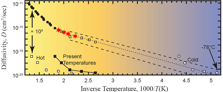
Figure 11. Arrhenius plot of measured data with the four lowest-temperature measured points marked as red stars. After Humphreys (2005).
(from this post – ed.)
From Poster 1:
More on my suspicion that the data from steps #16, 17, 18 are complete crap:
I looked up Farley et. al. (1999) on Farley's instrumentation and methods … Presumably this is the same instrumentation and technology that was used for the RATE study. …
In it they report:
Helium blanks in this device are generally low, in the range 1−4 fmol. The blanks do not scale strongly with either temperature (measured up to 750 °C) or holding time. …
What’s 1-4 fmol, you ask?
1-4 fmol = (1-4)·10-15 mole = (2.24- 8.96)·10-11 cc = 0.0224-0.0896 ncc at “STP” (standard temperature and pressure). That's the background. That's the reading that you get when you've gone to the greatest lengths you can go to to assure that there's zero helium present.
And how much helium was reported in steps 16, 17, 18?
0.00356, 0.000778, and 0.00203 ncc, respectively. In other words, at least an order of magnitude lower than machine background. And those are the three data points that Humphreys’ entire argument – that all of science is wrong, and contrary to all consilient science, for no apparent reason, radionuclide decay rates have jumped up and down by several orders of magnitude within the past few thousand years.
Can anyone explain to me why this is not complete garbage?
(from this post – ed.)
For those who are still interested in the instrument sensitivity issue, here is some more information. First, the reference cited by Poster 1 (Farley, 1999) is not the most informative because it deals primarily with the heating apparatus used by Farley and not the mass spectrometer analysis itself. More detailed information can be found in some of his later papers.
Helium diffusion from apatite: General behavior as illustrated by Durango fluorapatite
K. A. Farley
Helium was extracted from the apatites and accumulated in the chamber for periods ranging from 15 min to several weeks. The evolved helium was spiked with ~0.5 pmol of 99.3% pure 3He and measured on a Balzers Prisma quadrupole mass spectrometer after cryogenic concentration and purification. The amount of spike delivered was repeatedly cross-calibrated against a pipette that delivers a known amount of 4He determined to high precision and accuracy with a capacitance manometer. On the basis of reproducibility of standards the precision of He determinations presented here is better than 1% down to a few times the blank level. Blanks were essentially invariant with both time and temperature in the diffusion cell and were typically <1 fmol. All plotted data have been blank corrected; in general, the blank corrections are small (<2%), but in rare cases, blank correction is a substantial fraction of the total gas in a step. When blank corrections for a given data point exceeded 35% the point was ignored for plotting and interpretation. (Farley, 2000)
A few points to note. Farley measures the helium quantity using a method called “isotope dilution”, which is common in the geochronometry/thermochronometry business. Here is the issue. There is a difference between instrument sensitivity and the ability to measure quantity accurately. Let's use an example. Suppose we have an instrument with atomic level sensitivity (which AMS is not capable of doing!). Then, in theory, we could count atoms one-by-one. Let's suppose now we have 10,000 atoms in a box. Can we accurately count all of them? Well, our instrument could count all the atoms in principle, but in order to do so, we would have to insure that we could route every single atom through the system. In practice, the limiting factor is not the instrument sensitivity, but the ability to get every atom from the sample to the instrument. Isotope dilution provides the solution. In this method, a known quantity of material of a different isotopic concentration is added to the sample. Then, assuming that the sample and the isotope “spike” mix uniformly, one merely has to measure ratios instead of quantities, which is much easier to do.
Now back to Farley's measurements. He uses a 3He spike that is 99.3% pure, meaning that there is 0.7% “other stuff” in the spike, probably mostly 4He. This, undoubtedly, contributes to some of the background signal. Below is a table with some calculations and unit conversions.
| Sample | Concentration (fmol) | Concentration (ncc) | Atoms |
|---|---|---|---|
| Spike | 500.0000 | 11.20700 | 30,100·107 |
| Spike (He3) | 496.5000 | 11.12855 | 29,900·107 |
| Spike (other) | 3.5000 | 0.07845 | 211·107 |
| Blanks | 1.0000 | 0.02241 | 60.2·107 |
| Farley's Sample Reject Level (Blanks ÷ 0.35) |
2.8571 | 0.06404 | 172·107 |
| RATE #16 | 0.1588 | 0.00356 | 9.56·107 |
| RATE #17 | 0.0347 | 0.00078 | 2.09·107 |
| RATE #18 | 0.0906 | 0.00203 | 5.45·107 |
| RATE #19 | 0.1896 | 0.00425 | 11.4·107 |
Table 1. Instrument Background from Farley 2000.
As you can see, the blank concentration is on the same order as the "other stuff" in the spike, and the four low-temperature samples from Humphreys' RATE experiment are well below this background level. A later paper (Reiners, 2002) confirms this concentration level for experimental blanks.
4He released from the sample in each step was measured by a quadrupole mass spectrometer using 3He isotope dilution. He blanks were determined throughout the temperature range of our experiments and showed no time or temperature dependence; cold blanks were checked prior to each run and a typical blank of 0.02 ncc (STP) of 4He ( < 0.05% of typical 4He released at 500 C) was subtracted from each step.
(from this post – ed.)
Originally Posted by Poster 5:
so the amounts of material that RATE is relying on are even lower than the certainty of the purity of the spike, according to the data in that post.
That was my interpretation of the data.
(From this post - ed.) I have completed my preliminary analysis of the helium age data from the KTB drill hole Wolfe & Stockli (2010). Aside from some questions I have about the raw data in Table 1 for which I need to contact the authors, everything else is complete. My basic approach was based upon this statement in the paper:
If laboratory-derived zircon He diffusion kinetics apply in nature, then ZrHe ages from a 1-D sample array with a well-constrained thermal history should coincide with forward modeled ZrHe ages, or in other words a 1-D array of ages can be inverted to derived[sic] a geological estimate of the diffusion kinetics.
The authors demonstrated this agreement between “laboratory-derived zircon He diffusion kinetics” and “ZrHe ages from a 1-D sample array with a well-constrained thermal history” using forward modeling of the ZrHe ages (Figure 7). (Figure 7 from Wolfe & Stockli (2010) has been added here for convenience - ed.)
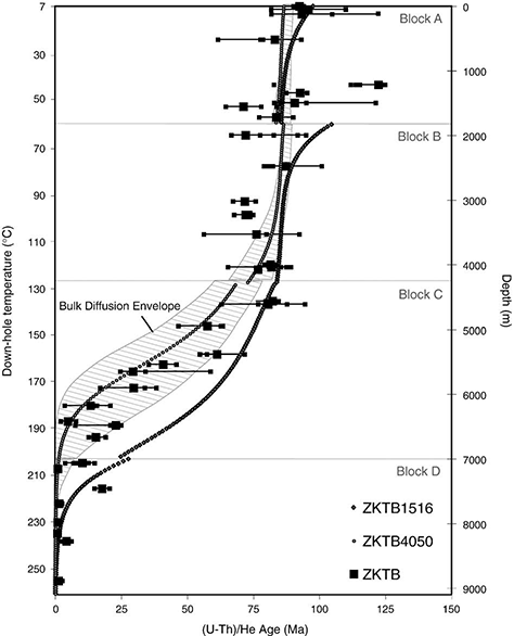
Figure 7 from Wolfe & Stockli (2010). Displays predicted down-hole zircon ages from modeling the thermal history seen in Fig. 4 (based on Wagner et al., 1997; Stockli and Farley, 2004) in comparison to ZrHe results from KTB drill hole from this study. ZrHe ages are plotted as individual ages (small grey square) and average ages (large grey square) with maximum age spread plotted as error. Hatched envelope models zircon bulk laboratory derived diffusion kinetics in a range from Ea 165–171 kJ/mol and D0 0.09–0.46 cm2 s−1 (Reiners et al., 2004; Reiners, 2005). White shapes (circle and square) reflect modeled results from laboratory derived diffusion kinetics from cycled step heating experiments on zircon from KTB drill hole. ZKTB4050-DE with Tc of ∼181 °C fits well with ZrHe ages, while ZKTB1516-DE with Tc of 215 °C sits well below ZrHe ages and but can account for anomalously old ZrHe ages that sit outside of bulk diffusion envelope.
Unfortunately, some participants on this thread were not able to follow their argument because of their inability to see the connection between ZrHe ages and helium diffusion kinetics. Therefore, I decided to pursue the alternate approach, which was suggested but not performed by the authors, namely, to invert the age data to derive “a geological estimate of the diffusion kinetics”. Here are the results.
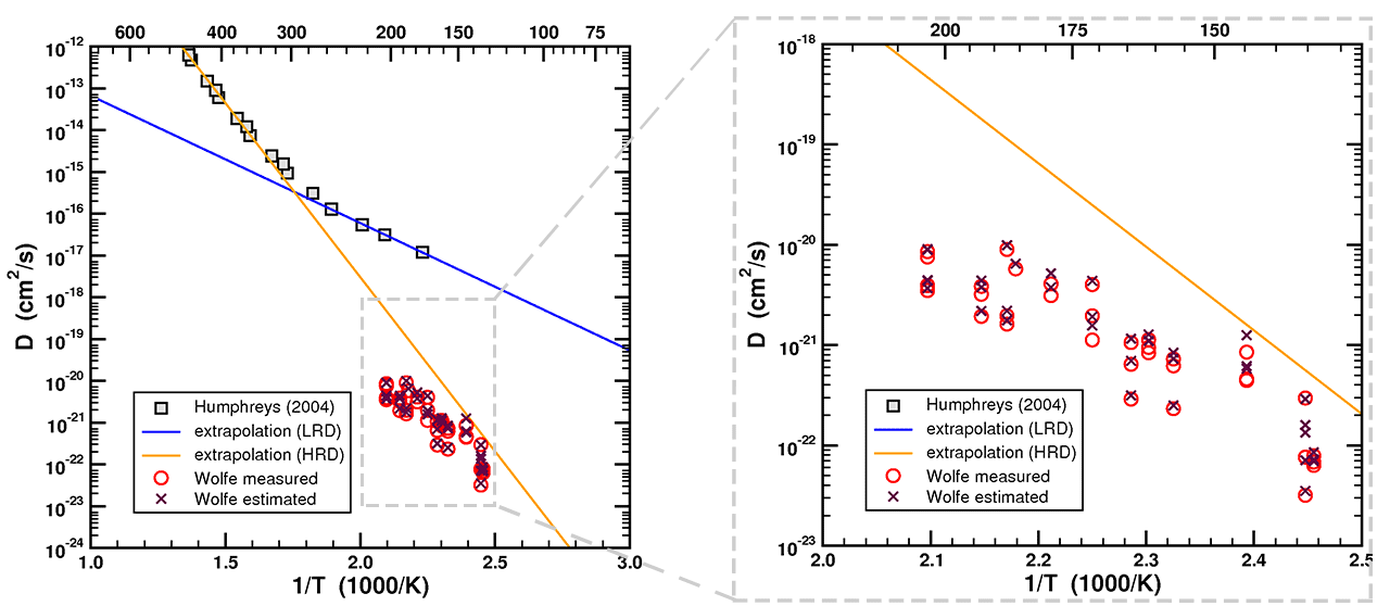
Figure 12. Arrhenius plot of data and fitted curve from Humphreys (2005) with single-domain straight-line fits of data from Reiners, et al. (2004) and back-calculated diffusivities from Wolfe & Stockli (2010).
(The figure above has been modified from the one presented in the discussion board thread. The purple X's indicate diffusivity calculated from Dr. Loechelt's estimate of radius from Ft, and are the same as presented previously. The red circles have been added to indicate diffusivity based on actual measurements (Wolfe 2011) - ed)
As you can see, the “laboratory-derived zircon He diffusion kinetics” from a number of sources such as Reiners (2004) or the extrapolation of the HRD of the RATE study (Humphreys, 2004) are a good predictor of the “geological estimate of the diffusion kinetics” derived by inverting the ZrHe ages. The extrapolation of the LRD of the RATE study, on the other hand, was a very poor predictor of the low-temperature helium diffusion kinetics.
(from this post – ed.)
Here are some of the technical details. First, my starting point was Table 1 from Wolfe & Stockli (2010). As I began to analyze the data, I found a number of inconsistencies. Not all of the data columns are independent. For instance, given the U and Th concentrations, the age, and the fraction of alpha particles remaining in the crystal, the He concentration can be calculated and compared with the reported value. Sometimes my calculation was consistent with the reported value. Other times it was way off. In those instances, however, I found that my calculation was consistent if I interpreted the reported He concentration in units of nmol/g instead of ncc/mg. This is the question that I need to address to the authors. (Since this was written Dr. Loechelt has contacted one of the authors of the referenced paper and verified that his conclusion that the reported He concentration is in units of nmol/g instead of ncc/mg is correct (Loechelt 2012) - ed) Assuming that my interpretation of the units is correct, I proceeded as follows.
I needed to know the fraction of He remaining, assuming some diffusion loss, and the effective radius of the crystal. Neither quantity was reported directly, so I calculated the total amount of helium generated for an accumulation time of 110 Ma using the reported values for U, Th, and FT. When I divided this quantity into the reported He concentration, I effectively obtained the equivalent of Gentry's Q/Q0 ratio. To obtain the effective radius of each sample, I started with the formula for FT (Equations 11 and 12 from Loechelt (2008) - ed.) and inverted the quadratic equation to obtain the surface-to-volume ratio. I then calculated the radius of the equivalent sphere with the same ratio. All of these calculations were done in an Excel spreadsheet. An abbreviated version of the table is given below.
Also, I calculated the temperature profile versus depth using the ≈27.5 C/km geothermal gradient and the mean annual surface temperature of ≈7 C reported in the paper. For the next step, all I needed was the temperature column, the Q/Q0 column, and the radius column of the table.
To perform the inversion of Q/Q0 to obtain the diffusivity D, I used a look-up table. I generated an array of 200 D·t (diffusivity x time) values (using equation 75 from Loechelt (2008) with C(0) = 0 and U = 1/t. - ed) with a density of 20 points per decade as the independent variable. These were used in my helium diffusion model with a 20 μm spherical radius to calculate a corresponding array of Q/Q0 values. I then normalized the D·t array to create an array of D/a2 values by dividing by the radius squared (400 μm) and the accumulation time (110 Ma) (The age of the zircons is bracketed by the 85-110 Ma ages above Partial Retention Zone. Calculating based on 85 Ma yielded Q/Q0 values greater than 100% (Loechelt (2012)), obviously impossible - ed). Now, swapping the roles of Q/Q0 and as dependent and independent variables, I had a look-up table whereby I could interpolate on Q/Q0 to find D/a2. I ran this interpolation on 37 samples from Table 1 of the Wolfe & Stockli (2010) paper. My selection criteria was to use samples from the helium partial retention zone (temperatures between 130 C and 210 C) which had Q/Q0 ratios between 5% and 95%. The result was an array of D/a2 values corresponding to each sample. Multiplying this array by the square of the effective spherical radius gave the diffusivity. I now had an array of D versus T values that I could plot on an Arrhenius graph.
(The table below has been extensively modified from the table published in the discussion thread. The added Width and Length columns are measurements of the sample from Wolfe (2011). β1 and Radius1 are calculated from Ft as discussed in the text and D1 is calculated from the diffusion model in Loechelt (2008) based on Radius1. β2 and Radius2 are calculated from the Width and Length, and D2 is calculated from the diffusion model in Loechelt (2008) based on the Radius2 column. The He column is the calculated amount produced, the He* column is the measured amount remaining. Most of the table columns are hidden to improve readability; if you want to see other columns click the “Show / Hide columns” button. Dr. Loechelt originally ordered the rows by depth, but I have moved the 37 values selected for calculating D to the top, with a light yellow background for the Sample column. - ed).
| Key to the color codes | |||||||||||||||||||
|
| ||||||||||||||||||
| Sample | Width (μm) | Length (μm) | Depth (m) | Temperature (C) |
Ft | c | b | a | β1 (1/μm) | β2 (1/μm) | Radius1 (μm) | Radius2 (μm) | Length/Width | Age (Ma) | ±(8%) (Ma) | Mass (μg) | U (ppm) | Th (ppm) | Th/U | e (U) |
U238 (ppm) | U235 (ppm) | Th232 (ppm) | Pb (ppm) | He (nmol/g) | He (ncc/mg) | He* (nmol/g) | He* (ncc/mg) | Q/Q0 | 1000/T (1/K) |
D1 (cm2/s) |
D2 (cm2/s) |
|---|---|---|---|---|---|---|---|---|---|---|---|---|---|---|---|---|---|---|---|---|---|---|---|---|---|---|---|---|---|---|---|---|
| ZKTB 4620-1 | 61.70 | 157.40 | -4620 | 134.1 | 0.700 | 0.300 | -4.415 | 5.206 | 0.074 | 0.078 | 40.3 | 38.7 | 2.55 | 79.6 | 6.4 | 2.80 | 115.70 | 66.50 | 2.40 | 95.50 | 1.98 | 0.09 | 0.36 | 2.12 | 55.04 | 1233.67 | 39.77 | 891.4 | 72.26 | 2.46 | 8.53·10-23 | 7.87·10-23 |
| ZKTB 4620-2 | 66.90 | 155.70 | -4620 | 134.1 | 0.720 | 0.280 | -4.406 | 5.182 | 0.069 | 0.073 | 43.4 | 41.3 | 2.33 | 84.4 | 6.7 | 3.20 | 143.00 | 71.90 | 1.40 | 154.80 | 2.44 | 0.12 | 0.39 | 2.57 | 68.93 | 1544.88 | 52.63 | 1179.6 | 76.36 | 2.46 | 6.96·10-23 | 6.31·10-23 |
| ZKTB 4620-3 | 66.40 | 151.30 | -4620 | 134.1 | 0.710 | 0.290 | -4.447 | 5.294 | 0.071 | 0.073 | 42.1 | 40.8 | 2.28 | 82.7 | 6.6 | 3.10 | 87.10 | 75.20 | 0.40 | 233.40 | 1.49 | 0.07 | 0.41 | 1.72 | 44.55 | 998.43 | 33.52 | 751.3 | 75.25 | 2.46 | 7.24·10-23 | 6.82·10-23 |
| ZKTB 4668-1 | 78.38 | 263.96 | -4668 | 135.4 | 0.750 | 0.250 | -4.435 | 5.260 | 0.061 | 0.059 | 49.4 | 51.2 | 3.37 | 87.6 | 7.0 | 4.80 | 63.00 | 47.20 | 0.70 | 159.50 | 1.08 | 0.05 | 0.26 | 1.21 | 33.27 | 745.80 | 26.23 | 587.9 | 78.83 | 2.45 | 7.10·10-23 | 7.63·10-23 |
| ZKTB 4668-2 | 72.25 | 184.38 | -4668 | 135.4 | 0.730 | 0.270 | -4.371 | 5.086 | 0.067 | 0.066 | 44.8 | 45.3 | 2.55 | 62.9 | 5.0 | 3.90 | 61.00 | 14.10 | 0.20 | 104.40 | 1.04 | 0.05 | 0.08 | 1.01 | 28.10 | 629.90 | 16.02 | 359.1 | 57.00 | 2.45 | 2.89·10-22 | 2.96·10-22 |
| ZKTB 4668-3 | 82.58 | 187.08 | -4668 | 135.4 | 0.770 | 0.230 | -4.378 | 5.104 | 0.056 | 0.059 | 53.4 | 50.7 | 2.27 | 94.4 | 7.6 | 7.50 | 92.00 | 25.70 | 0.90 | 131.70 | 1.57 | 0.07 | 0.14 | 1.55 | 45.19 | 1012.87 | 38.81 | 869.9 | 85.88 | 2.45 | 3.51·10-23 | 3.18·10-23 |
| ZKTB 4668-4 | -4668 | 135.4 | 0.750 | 0.250 | -4.383 | 5.118 | 0.061 | 48.8 | 76.8 | 6.1 | 4.50 | 60.50 | 19.20 | 1.20 | 73.80 | 1.03 | 0.05 | 0.10 | 1.03 | 29.19 | 654.23 | 20.17 | 452.1 | 69.10 | 2.45 | 1.59·10-22 | ||||||
| ZKTB 4668-5 | -4668 | 135.4 | 0.770 | 0.230 | -4.366 | 5.072 | 0.056 | 53.2 | 80.9 | 6.5 | 5.90 | 128.90 | 24.80 | 0.60 | 64.20 | 2.20 | 0.10 | 0.14 | 2.12 | 62.10 | 1391.82 | 45.65 | 1023.2 | 73.52 | 2.45 | 1.34·10-22 | ||||||
| ZKTB 5008-1 | 80.70 | 206.40 | -5008 | 144.7 | 0.800 | 0.200 | -4.339 | 4.999 | 0.049 | 0.059 | 61.4 | 50.6 | 2.56 | 46.5 | 3.7 | 6.30 | 85.00 | 0.80 | 0.40 | 65.00 | 1.45 | 0.07 | 0.00 | 1.32 | 40.79 | 914.21 | 16.60 | 372.1 | 40.70 | 2.39 | 1.25·10-21 | 8.51·10-22 |
| ZKTB 5008-2 | 84.60 | 204.00 | -5008 | 144.7 | 0.800 | 0.200 | -4.376 | 5.099 | 0.048 | 0.057 | 61.9 | 52.6 | 2.41 | 62.6 | 5.0 | 6.80 | 150.90 | 40.20 | 0.90 | 134.60 | 2.58 | 0.12 | 0.22 | 2.54 | 76.79 | 1721.11 | 42.30 | 948.1 | 55.09 | 2.39 | 6.16·10-22 | 4.43·10-22 |
| ZKTB 5008-3 | 84.40 | 292.50 | -5008 | 144.7 | 0.800 | 0.200 | -4.404 | 5.176 | 0.048 | 0.054 | 62.3 | 55.3 | 3.47 | 63.3 | 5.1 | 9.70 | 105.10 | 50.90 | 0.90 | 87.10 | 1.80 | 0.09 | 0.28 | 1.88 | 56.07 | 1256.68 | 31.60 | 708.3 | 56.36 | 2.39 | 5.82·10-22 | 4.58·10-22 |
| ZKTB 5608-1 | 73.00 | 240.70 | -5608 | 161.2 | 0.760 | 0.240 | -4.338 | 4.997 | 0.059 | 0.063 | 50.5 | 47.5 | 3.30 | 35.3 | 2.8 | 6.00 | 127.30 | 0.70 | 0.00 | 160.10 | 2.18 | 0.10 | 0.00 | 1.98 | 57.98 | 1299.50 | 18.57 | 416.2 | 32.03 | 2.30 | 1.28·10-21 | 1.13·10-21 |
| ZKTB 5608-2 | 72.30 | 200.40 | -5608 | 161.2 | 0.770 | 0.230 | -4.339 | 4.998 | 0.057 | 0.065 | 52.9 | 45.9 | 2.77 | 41.1 | 3.3 | 4.90 | 129.70 | 0.80 | 0.00 | 116.90 | 2.22 | 0.11 | 0.00 | 2.01 | 59.86 | 1341.64 | 22.11 | 495.6 | 36.94 | 2.30 | 1.11·10-21 | 8.37·10-22 |
| ZKTB 5608-3 | 88.20 | 198.80 | -5608 | 161.2 | 0.790 | 0.210 | -4.338 | 4.997 | 0.051 | 0.055 | 58.3 | 54.1 | 2.25 | 45.8 | 3.7 | 7.20 | 153.70 | 0.60 | 0.00 | 120.70 | 2.63 | 0.13 | 0.00 | 2.39 | 72.74 | 1630.32 | 30.01 | 672.6 | 41.26 | 2.30 | 1.10·10-21 | 9.46·10-22 |
| ZKTB 5450-1 | 79.40 | 247.40 | -5450 | 156.9 | 0.770 | 0.230 | -4.369 | 5.080 | 0.056 | 0.058 | 53.3 | 51.3 | 3.12 | 71.6 | 5.7 | 7.30 | 151.60 | 32.60 | 0.80 | 112.40 | 2.59 | 0.12 | 0.18 | 2.51 | 73.40 | 1645.29 | 47.80 | 1071.4 | 65.12 | 2.33 | 2.50·10-22 | 2.32·10-22 |
| ZKTB 5450-2 | 90.70 | 224.90 | -5450 | 156.9 | 0.800 | 0.200 | -4.340 | 5.001 | 0.049 | 0.053 | 61.4 | 56.6 | 2.48 | 57.3 | 4.6 | 8.60 | 112.00 | 1.70 | 0.50 | 43.10 | 1.91 | 0.09 | 0.01 | 1.74 | 53.82 | 1206.24 | 27.77 | 622.4 | 51.60 | 2.33 | 7.31·10-22 | 6.20·10-22 |
| ZKTB 5450-3 | 93.50 | 214.10 | -5450 | 156.9 | 0.800 | 0.200 | -4.370 | 5.085 | 0.048 | 0.052 | 61.9 | 57.6 | 2.29 | 54.6 | 4.4 | 8.70 | 41.00 | 9.30 | 0.50 | 104.90 | 0.70 | 0.03 | 0.05 | 0.68 | 20.68 | 463.53 | 10.17 | 228.0 | 49.18 | 2.33 | 8.39·10-22 | 7.26·10-22 |
| ZKTB 5720-1 | 61.60 | 206.80 | -5720 | 164.3 | 0.710 | 0.290 | -4.431 | 5.249 | 0.072 | 0.075 | 42.0 | 40.2 | 3.36 | 58.7 | 4.7 | 3.60 | 95.90 | 68.10 | 1.20 | 129.90 | 1.64 | 0.08 | 0.37 | 1.82 | 47.57 | 1066.30 | 25.25 | 566.0 | 53.08 | 2.29 | 3.15·10-22 | 2.89·10-22 |
| ZKTB 5720-2 | 58.30 | 135.40 | -5720 | 164.3 | 0.680 | 0.320 | -4.433 | 5.256 | 0.080 | 0.083 | 37.6 | 36.0 | 2.32 | 24.6 | 2.0 | 2.10 | 49.50 | 36.30 | 2.60 | 153.80 | 0.85 | 0.04 | 0.20 | 0.94 | 23.63 | 529.60 | 5.24 | 117.4 | 22.18 | 2.29 | 1.16·10-21 | 1.06·10-21 |
| ZKTB 5720-3 | 55.80 | 139.40 | -5720 | 164.3 | 0.670 | 0.330 | -4.424 | 5.232 | 0.083 | 0.086 | 36.3 | 34.9 | 2.50 | 34.1 | 2.7 | 2.00 | 80.70 | 52.90 | 2.80 | 137.10 | 1.38 | 0.07 | 0.29 | 1.51 | 37.36 | 837.41 | 11.53 | 258.4 | 30.86 | 2.29 | 6.97·10-22 | 6.43·10-22 |
| ZKTB 5975-1 | 96.44 | 238.01 | -5975 | 171.3 | 0.790 | 0.210 | -4.431 | 5.250 | 0.050 | 0.050 | 59.5 | 60.1 | 2.47 | 33.8 | 0.2 | 10.00 | 78.70 | 56.30 | 0.70 | 57.80 | 1.34 | 0.06 | 0.31 | 1.50 | 43.49 | 974.69 | 13.20 | 295.9 | 30.35 | 2.25 | 1.92·10-21 | 1.96·10-21 |
| ZKTB 5975-2 | 91.14 | 219.47 | -5975 | 171.3 | 0.790 | 0.210 | -4.397 | 5.157 | 0.051 | 0.053 | 59.1 | 56.6 | 2.41 | 16.9 | 0.1 | 10.00 | 39.50 | 16.90 | 0.40 | 92.90 | 0.67 | 0.03 | 0.09 | 0.69 | 20.56 | 460.82 | 3.12 | 69.9 | 15.18 | 2.25 | 4.37·10-21 | 4.01·10-21 |
| ZKTB 5975-3 | 79.61 | 208.29 | -5975 | 171.3 | 0.790 | 0.210 | -4.409 | 5.191 | 0.051 | 0.060 | 59.2 | 50.1 | 2.62 | 38.2 | 0.2 | 10.00 | 31.40 | 16.60 | 0.50 | 75.30 | 0.54 | 0.03 | 0.09 | 0.57 | 16.70 | 374.24 | 5.74 | 128.7 | 34.38 | 2.25 | 1.57·10-21 | 1.12·10-21 |
| ZKTB 6255-1 | 90.80 | 206.40 | -6255 | 179.0 | 0.800 | 0.200 | -4.339 | 4.998 | 0.049 | 0.054 | 61.4 | 55.8 | 2.27 | 20.8 | 1.7 | 7.90 | 151.90 | 1.10 | 0.50 | 43.30 | 2.60 | 0.12 | 0.01 | 2.36 | 72.85 | 1632.91 | 13.60 | 304.8 | 18.67 | 2.21 | 3.77·10-21 | 3.11·10-21 |
| ZKTB 6255-2 | 86.30 | 227.00 | -6255 | 179.0 | 0.800 | 0.200 | -4.339 | 4.998 | 0.049 | 0.055 | 61.4 | 54.4 | 2.63 | 15.6 | 1.3 | 7.90 | 114.20 | 0.90 | 0.30 | 35.30 | 1.95 | 0.09 | 0.00 | 1.77 | 54.78 | 1227.82 | 7.60 | 170.3 | 13.87 | 2.21 | 5.19·10-21 | 4.07·10-21 |
| ZKTB 6500-2 | 76.60 | 150.60 | -6500 | 185.8 | 0.750 | 0.250 | -4.362 | 5.061 | 0.062 | 0.065 | 48.6 | 45.8 | 1.97 | 7.8 | 0.6 | 4.10 | 5.50 | 0.90 | 1.90 | 35.00 | 0.09 | 0.00 | 0.00 | 0.09 | 2.56 | 57.47 | 0.18 | 4.0 | 7.02 | 2.18 | 6.48·10-21 | 5.76·10-21 |
| ZKTB 6562-1 | 71.20 | 173.90 | -6562 | 187.5 | 0.740 | 0.260 | -4.396 | 5.155 | 0.064 | 0.068 | 46.9 | 44.3 | 2.44 | 20.8 | 1.7 | 4.10 | 139.00 | 58.70 | 0.40 | 5.70 | 2.38 | 0.11 | 0.32 | 2.44 | 67.69 | 1517.20 | 12.66 | 283.8 | 18.70 | 2.17 | 2.20·10-21 | 1.96·10-21 |
| ZKTB 6562-2 | 94.90 | 178.60 | -6562 | 187.5 | 0.790 | 0.210 | -4.395 | 5.152 | 0.051 | 0.053 | 59.0 | 56.2 | 1.88 | 7.5 | 0.6 | 7.50 | 76.60 | 31.60 | 0.40 | 15.90 | 1.31 | 0.06 | 0.17 | 1.34 | 39.74 | 890.72 | 2.69 | 60.3 | 6.77 | 2.17 | 9.90·10-21 | 8.98·10-21 |
| ZKTB 6562-3 | 71.10 | 189.50 | -6562 | 187.5 | 0.740 | 0.260 | -4.387 | 5.131 | 0.064 | 0.067 | 46.8 | 44.9 | 2.67 | 24.9 | 2.0 | 4.50 | 135.90 | 48.10 | 0.40 | 11.00 | 2.32 | 0.11 | 0.26 | 2.34 | 65.21 | 1461.62 | 14.68 | 329.0 | 22.51 | 2.17 | 1.76·10-21 | 1.62·10-21 |
| ZKTB 6750-1 | 74.20 | 191.00 | -6750 | 192.6 | 0.760 | 0.240 | -4.344 | 5.014 | 0.059 | 0.064 | 50.6 | 46.6 | 2.57 | 14.4 | 1.2 | 4.90 | 407.40 | 18.20 | 0.70 | 83.80 | 6.96 | 0.33 | 0.10 | 6.40 | 187.26 | 4197.19 | 24.25 | 543.5 | 12.95 | 2.15 | 3.78·10-21 | 3.21·10-21 |
| ZKTB 6750-2 | 79.40 | 157.00 | -6750 | 192.6 | 0.760 | 0.240 | -4.366 | 5.072 | 0.059 | 0.063 | 50.8 | 47.5 | 1.98 | 12.5 | 1.0 | 4.60 | 108.50 | 21.00 | 1.70 | 146.90 | 1.85 | 0.09 | 0.11 | 1.78 | 51.60 | 1156.63 | 5.81 | 130.2 | 11.26 | 2.15 | 4.41·10-21 | 3.85·10-21 |
| ZKTB 6750-3 | 69.00 | 147.90 | -6750 | 192.6 | 0.730 | 0.270 | -4.361 | 5.058 | 0.067 | 0.071 | 44.7 | 42.0 | 2.14 | 19.0 | 1.5 | 3.30 | 42.20 | 6.60 | 1.30 | 127.80 | 0.72 | 0.03 | 0.04 | 0.69 | 19.12 | 428.48 | 3.28 | 73.5 | 17.16 | 2.15 | 2.19·10-21 | 1.93·10-21 |
| ZKTB 7152-1 | 81.60 | 215.90 | -7152 | 203.7 | 0.780 | 0.220 | -4.369 | 5.081 | 0.054 | 0.058 | 55.9 | 51.5 | 2.65 | 7.5 | 0.6 | 6.70 | 117.50 | 25.60 | 0.50 | 113.40 | 2.01 | 0.10 | 0.14 | 1.95 | 57.67 | 1292.59 | 3.89 | 87.2 | 6.75 | 2.10 | 8.89·10-21 | 7.55·10-21 |
| ZKTB 7152-2 | 71.50 | 168.70 | -7152 | 203.7 | 0.740 | 0.260 | -4.365 | 5.070 | 0.064 | 0.068 | 46.6 | 44.2 | 2.36 | 10.6 | 0.8 | 4.00 | 234.30 | 43.90 | 1.40 | 43.70 | 4.00 | 0.19 | 0.24 | 3.85 | 108.35 | 2428.57 | 10.35 | 232.0 | 9.55 | 2.10 | 4.37·10-21 | 3.94·10-21 |
| ZKTB 7152-3 | 77.10 | 187.30 | -7152 | 203.7 | 0.760 | 0.240 | -4.386 | 5.127 | 0.059 | 0.063 | 51.1 | 48.0 | 2.43 | 12.5 | 1.0 | 5.20 | 134.40 | 46.20 | 1.90 | 189.60 | 2.30 | 0.11 | 0.25 | 2.31 | 66.09 | 1481.26 | 7.45 | 167.0 | 11.27 | 2.10 | 4.44·10-21 | 3.92·10-21 |
| ZKTB 7154-1 | 84.00 | 187.10 | -7154 | 203.7 | 0.770 | 0.230 | -4.340 | 5.002 | 0.057 | 0.058 | 52.9 | 51.5 | 2.23 | 14.9 | 1.2 | 6.10 | 115.90 | 2.00 | 0.30 | 244.40 | 1.98 | 0.09 | 0.01 | 1.81 | 53.63 | 1202.02 | 7.74 | 173.5 | 14.43 | 2.10 | 3.69·10-21 | 3.49·10-21 |
| ZKTB 7154-2 | 88.10 | 194.80 | -7154 | 203.7 | 0.780 | 0.220 | -4.339 | 4.999 | 0.054 | 0.056 | 55.5 | 53.9 | 2.21 | 6.8 | 0.5 | 7.00 | 170.60 | 1.40 | 0.30 | 145.00 | 2.92 | 0.14 | 0.01 | 2.65 | 79.79 | 1788.49 | 5.22 | 117.0 | 6.54 | 2.10 | 9.05·10-21 | 8.54·10-21 |
| ZKTBQ-1 | 59.50 | 138.60 | 0 | 7.0 | 0.690 | 0.310 | -4.371 | 5.087 | 0.078 | 0.082 | 38.5 | 36.7 | 2.33 | 92.9 | 7.4 | 2.30 | 265.80 | 62.00 | 0.20 | 280.09 | 4.54 | 0.22 | 0.34 | 4.42 | 115.80 | 2595.54 | 97.89 | 2194.1 | 84.53 | |||
| ZKTBQ-2 | 69.10 | 179.00 | 0 | 7.0 | 0.730 | 0.270 | -4.385 | 5.124 | 0.067 | 0.069 | 44.9 | 43.4 | 2.59 | 90.1 | 7.2 | 4.00 | 915.00 | 307.00 | 0.30 | 985.69 | 15.64 | 0.74 | 1.68 | 15.69 | 431.38 | 9669.00 | 354.21 | 7939.3 | 82.11 | |||
| ZKTBQ-3 | 81.30 | 167.20 | 0 | 7.0 | 0.760 | 0.240 | -4.396 | 5.154 | 0.059 | 0.061 | 51.2 | 49.0 | 2.06 | 93.9 | 7.5 | 5.10 | 1056.60 | 443.40 | 0.40 | 1158.65 | 18.05 | 0.86 | 2.42 | 18.55 | 528.15 | 11837.84 | 450.17 | 10090.1 | 85.24 | |||
| ZKTB 52-2 | 58.30 | 113.14 | -52 | 8.4 | 0.680 | 0.320 | -4.364 | 5.066 | 0.081 | 0.086 | 37.1 | 34.8 | 1.94 | 109.9 | 8.8 | 1.80 | 196.80 | 35.10 | 0.18 | 204.92 | 3.36 | 0.16 | 0.19 | 3.22 | 83.46 | 1870.67 | 83.93 | 1881.2 | 100.56 | |||
| ZKTB 52-3 | 52.90 | 112.90 | -52 | 8.4 | 0.660 | 0.340 | -4.348 | 5.023 | 0.087 | 0.093 | 34.5 | 32.1 | 2.13 | 81.6 | 6.5 | 1.50 | 318.90 | 22.10 | 0.07 | 324.03 | 5.45 | 0.26 | 0.12 | 5.05 | 128.02 | 2869.53 | 95.43 | 2138.9 | 74.54 | |||
| ZKTB 115-7 | 95.75 | 141.09 | -115 | 10.2 | 0.780 | 0.220 | -4.370 | 5.083 | 0.054 | 0.056 | 55.9 | 53.6 | 1.47 | 122.2 | 9.8 | 6.00 | 27.80 | 6.20 | 0.90 | 29.21 | 0.48 | 0.02 | 0.03 | 0.46 | 13.66 | 306.17 | 15.21 | 340.9 | 111.35 | |||
| ZKTB 125-2 | 69.98 | 151.58 | -125 | 10.4 | 0.700 | 0.300 | -4.395 | 5.150 | 0.075 | 0.070 | 40.1 | 42.6 | 2.17 | 81.7 | 6.5 | 3.50 | 27.60 | 11.30 | 1.10 | 30.17 | 0.47 | 0.02 | 0.06 | 0.48 | 12.68 | 284.19 | 9.80 | 219.7 | 77.29 | |||
| ZKTB 125-3 | 55.80 | 148.19 | -125 | 10.4 | 0.700 | 0.300 | -4.385 | 5.125 | 0.075 | 0.085 | 40.0 | 35.2 | 2.66 | 104.7 | 8.4 | 2.10 | 47.30 | 15.90 | 1.20 | 50.97 | 0.81 | 0.04 | 0.09 | 0.81 | 21.39 | 479.35 | 19.70 | 441.6 | 92.11 | |||
| ZKTB 525-1 | 72.70 | 181.50 | -525 | 21.4 | 0.700 | 0.300 | -4.438 | 5.268 | 0.074 | 0.066 | 40.5 | 45.4 | 2.50 | 93.0 | 7.4 | 4.50 | 159.40 | 123.40 | 2.00 | 187.77 | 2.72 | 0.13 | 0.67 | 3.07 | 78.97 | 1769.99 | 70.40 | 1577.9 | 89.15 | |||
| ZKTB 525-2 | 81.70 | 174.20 | -525 | 21.4 | 0.700 | 0.300 | -4.340 | 5.001 | 0.076 | 0.060 | 39.6 | 49.6 | 2.13 | 77.6 | 6.2 | 5.40 | 146.60 | 2.20 | 0.70 | 147.08 | 2.51 | 0.12 | 0.01 | 2.28 | 61.63 | 1381.46 | 44.40 | 995.2 | 72.04 | |||
| ZKTB 525-3 | 94.00 | 196.60 | -525 | 21.4 | 0.800 | 0.200 | -4.370 | 5.085 | 0.048 | 0.053 | 61.9 | 56.9 | 2.09 | 78.5 | 6.3 | 8.10 | 200.50 | 45.40 | 1.10 | 210.96 | 3.43 | 0.16 | 0.25 | 3.33 | 101.12 | 2266.55 | 71.10 | 1593.6 | 70.31 | |||
| ZKTB 525-4 | 52.60 | 118.20 | -525 | 21.4 | 0.660 | 0.340 | -4.351 | 5.033 | 0.087 | 0.093 | 34.5 | 32.3 | 2.25 | 61.5 | 4.9 | 1.50 | 19.60 | 1.80 | 0.00 | 19.99 | 0.33 | 0.02 | 0.01 | 0.31 | 7.91 | 177.29 | 4.29 | 96.2 | 54.24 | |||
| ZKTB 1230-1 | 86.00 | 233.90 | -1230 | 40.8 | 0.780 | 0.220 | -4.392 | 5.143 | 0.053 | 0.055 | 56.1 | 54.5 | 2.72 | 115.2 | 9.2 | 8.00 | 133.40 | 51.90 | 0.39 | 145.37 | 2.28 | 0.11 | 0.28 | 2.32 | 67.99 | 1523.84 | 72.09 | 1615.9 | 106.04 | |||
| ZKTB 1230-2 | 119.80 | 261.10 | -1230 | 40.8 | 0.830 | 0.170 | -4.411 | 5.195 | 0.040 | 0.041 | 74.1 | 73.1 | 2.18 | 113.6 | 9.1 | 17.40 | 112.60 | 61.00 | 0.54 | 126.62 | 1.92 | 0.09 | 0.33 | 2.04 | 63.08 | 1413.82 | 65.96 | 1478.4 | 104.57 | |||
| ZKTB 1230-3 | 115.00 | 291.90 | -1230 | 40.8 | 0.830 | 0.170 | -4.413 | 5.202 | 0.040 | 0.042 | 74.2 | 72.1 | 2.54 | 124.7 | 10.0 | 17.90 | 110.30 | 62.00 | 0.56 | 124.53 | 1.88 | 0.09 | 0.34 | 2.01 | 62.05 | 1390.84 | 71.12 | 1594.0 | 114.61 | |||
| ZKTB 1230-4 | 75.00 | 220.10 | -1230 | 40.8 | 0.760 | 0.240 | -4.383 | 5.118 | 0.059 | 0.062 | 51.0 | 48.1 | 2.93 | 122.5 | 9.8 | 5.80 | 47.60 | 15.10 | 51.03 | 51.03 | 0.81 | 0.04 | 0.08 | 0.81 | 23.27 | 521.58 | 25.81 | 578.5 | 110.91 | |||
| ZKTB 1230-5 | 92.10 | 174.10 | -1230 | 40.8 | 0.790 | 0.210 | -4.345 | 5.015 | 0.051 | 0.055 | 58.4 | 54.6 | 1.89 | 82.7 | 6.6 | 6.90 | 12.40 | 0.60 | 12.54 | 12.54 | 0.21 | 0.01 | 0.00 | 0.20 | 5.93 | 132.91 | 4.44 | 99.5 | 74.88 | |||
| ZKTB 1358-1 | 74.83 | 187.27 | -1358 | 44.3 | 0.760 | 0.240 | -4.339 | 4.998 | 0.059 | 0.064 | 50.5 | 46.8 | 2.50 | 87.4 | 7.0 | 4.90 | 80.90 | 0.50 | 0.00 | 80.99 | 1.38 | 0.07 | 0.00 | 1.26 | 36.85 | 825.98 | 29.08 | 651.8 | 78.91 | |||
| ZKTB 1358-2 | 62.57 | 166.16 | -1358 | 44.3 | 0.720 | 0.280 | -4.340 | 5.001 | 0.070 | 0.076 | 42.7 | 39.5 | 2.66 | 95.2 | 7.6 | 3.00 | 69.00 | 1.00 | 0.00 | 69.26 | 1.18 | 0.06 | 0.01 | 1.07 | 29.83 | 668.71 | 25.66 | 575.1 | 86.01 | |||
| ZKTB 1358-3 | 63.10 | 132.05 | -1358 | 44.3 | 0.710 | 0.290 | -4.360 | 5.055 | 0.073 | 0.079 | 41.3 | 38.2 | 2.09 | 95.2 | 7.6 | 2.40 | 59.80 | 8.90 | 0.10 | 61.85 | 1.02 | 0.05 | 0.05 | 0.97 | 26.30 | 589.54 | 22.57 | 505.9 | 85.81 | |||
| ZKTB 1516-1 | 83.30 | 155.80 | -1516 | 48.7 | 0.770 | 0.230 | -4.340 | 5.001 | 0.057 | 0.061 | 52.9 | 49.3 | 1.87 | 82.8 | 6.6 | 5.00 | 13.40 | 0.20 | 0.00 | 13.48 | 0.23 | 0.01 | 0.00 | 0.21 | 6.20 | 138.90 | 4.66 | 104.4 | 75.20 | |||
| ZKTB 1516-2 | 70.60 | 184.30 | -1516 | 48.7 | 0.750 | 0.250 | -4.339 | 4.999 | 0.062 | 0.068 | 48.3 | 44.4 | 2.61 | 90.6 | 7.2 | 4.30 | 32.70 | 0.30 | 0.00 | 32.74 | 0.56 | 0.03 | 0.00 | 0.51 | 14.71 | 329.70 | 12.02 | 269.4 | 81.72 | |||
| ZKTB 1516-3 | 67.20 | 140.80 | -1516 | 48.7 | 0.730 | 0.270 | -4.344 | 5.013 | 0.067 | 0.074 | 44.5 | 40.7 | 2.10 | 85.1 | 6.8 | 3.00 | 18.80 | 0.80 | 0.00 | 18.99 | 0.32 | 0.02 | 0.00 | 0.30 | 8.30 | 185.95 | 6.37 | 142.8 | 76.78 | |||
| ZKTB 1516-4 | 87.60 | 162.60 | -1516 | 48.7 | 0.770 | 0.230 | -4.399 | 5.163 | 0.056 | 0.058 | 53.6 | 51.8 | 1.86 | 121.2 | 9.7 | 5.80 | 49.00 | 21.90 | 0.60 | 54.07 | 0.84 | 0.04 | 0.12 | 0.87 | 24.96 | 559.46 | 27.60 | 618.6 | 110.58 | |||
| ZKTB 1575-1 | 73.90 | 195.90 | -1575 | 50.3 | 0.760 | 0.240 | -4.339 | 4.999 | 0.059 | 0.064 | 50.5 | 46.6 | 2.65 | 77.9 | 6.2 | 5.00 | 22.60 | 0.20 | 0.01 | 22.65 | 0.39 | 0.02 | 0.00 | 0.35 | 10.30 | 230.89 | 7.31 | 163.8 | 70.94 | |||
| ZKTB 1575-2 | 69.30 | 198.40 | -1575 | 50.3 | 0.750 | 0.250 | -4.340 | 5.003 | 0.062 | 0.068 | 48.4 | 44.2 | 2.86 | 64.4 | 5.2 | 4.40 | 128.30 | 2.30 | 0.02 | 128.87 | 2.19 | 0.10 | 0.01 | 2.00 | 57.83 | 1296.26 | 33.84 | 758.4 | 58.51 | |||
| ZKTB 1575-4 | 75.10 | 200.70 | -1575 | 50.3 | 0.760 | 0.240 | -4.362 | 5.061 | 0.059 | 0.063 | 50.8 | 47.4 | 2.67 | 83.7 | 6.7 | 5.30 | 261.90 | 43.00 | 0.16 | 271.78 | 4.48 | 0.21 | 0.23 | 4.27 | 123.74 | 2773.43 | 94.36 | 2115.0 | 76.26 | |||
| ZKTB 1740-1 | 68.13 | 145.38 | -1740 | 54.9 | 0.730 | 0.270 | -4.372 | 5.089 | 0.067 | 0.072 | 44.8 | 41.4 | 2.13 | 140.4 | 11.2 | 3.10 | 143.50 | 34.30 | 0.20 | 151.43 | 2.45 | 0.12 | 0.19 | 2.39 | 66.23 | 1484.43 | 83.96 | 1881.9 | 126.77 | |||
| ZKTB 1740-2 | 72.07 | 158.82 | -1740 | 54.9 | 0.740 | 0.260 | -4.347 | 5.021 | 0.065 | 0.068 | 46.4 | 44.1 | 2.20 | 77.1 | 6.2 | 3.80 | 76.60 | 4.90 | 0.10 | 77.74 | 1.31 | 0.06 | 0.03 | 1.21 | 34.44 | 771.85 | 24.16 | 541.5 | 70.16 | |||
| ZKTB 1740-3 | 69.40 | 147.52 | -1740 | 54.9 | 0.730 | 0.270 | -4.364 | 5.067 | 0.067 | 0.071 | 44.7 | 42.1 | 2.13 | 89.9 | 7.2 | 3.30 | 159.00 | 28.70 | 0.20 | 165.59 | 2.72 | 0.13 | 0.16 | 2.61 | 72.42 | 1623.28 | 59.02 | 1322.9 | 81.49 | |||
| ZKTB 2020-1 | 64.41 | 194.57 | -2020 | 62.6 | 0.700 | 0.300 | -4.353 | 5.037 | 0.076 | 0.072 | 39.7 | 41.4 | 3.02 | 77.5 | 6.2 | 3.80 | 251.90 | 26.30 | 1.30 | 257.99 | 4.30 | 0.20 | 0.14 | 4.03 | 108.13 | 2423.60 | 78.80 | 1766.2 | 72.88 | |||
| ZKTB 2020-2 | 61.42 | 158.53 | -2020 | 62.6 | 0.700 | 0.300 | -4.390 | 5.139 | 0.075 | 0.078 | 40.1 | 38.6 | 2.58 | 66.6 | 5.3 | 2.80 | 127.70 | 48.10 | 1.80 | 138.79 | 2.18 | 0.10 | 0.26 | 2.21 | 58.25 | 1305.61 | 35.30 | 791.2 | 60.60 | |||
| ZKTB 2020-3 | 73.00 | 153.14 | -2020 | 62.6 | 0.740 | 0.260 | -4.339 | 4.998 | 0.065 | 0.068 | 46.3 | 44.2 | 2.10 | 94.8 | 7.6 | 3.80 | 315.70 | 2.50 | 0.30 | 316.27 | 5.39 | 0.26 | 0.01 | 4.91 | 140.08 | 3139.71 | 128.89 | 2888.9 | 92.01 | |||
| ZKTB 2020-4 | 68.88 | 142.15 | -2020 | 62.6 | 0.720 | 0.280 | -4.340 | 5.000 | 0.070 | 0.072 | 42.7 | 41.6 | 2.06 | 91.7 | 7.3 | 3.10 | 246.50 | 3.10 | 0.40 | 247.25 | 4.21 | 0.20 | 0.02 | 3.84 | 106.53 | 2387.86 | 97.73 | 2190.5 | 91.74 | |||
| ZKTB 2507-1 | 63.30 | 188.10 | -2507 | 75.9 | 0.720 | 0.280 | -4.345 | 5.016 | 0.070 | 0.074 | 42.8 | 40.6 | 2.97 | 82.3 | 6.6 | 3.50 | 27.20 | 1.40 | 0.90 | 27.50 | 0.46 | 0.02 | 0.01 | 0.43 | 11.86 | 265.90 | 8.88 | 199.0 | 74.85 | |||
| ZKTB 2507-2 | 73.80 | 223.00 | -2507 | 75.9 | 0.760 | 0.240 | -4.348 | 5.023 | 0.059 | 0.063 | 50.6 | 47.5 | 3.02 | 78.9 | 6.3 | 5.60 | 19.10 | 1.30 | 0.80 | 19.36 | 0.33 | 0.02 | 0.01 | 0.30 | 8.83 | 197.85 | 6.29 | 141.0 | 71.26 | |||
| ZKTB 2507-3 | 61.60 | 161.30 | -2507 | 75.9 | 0.710 | 0.290 | -4.347 | 5.021 | 0.073 | 0.077 | 41.2 | 38.8 | 2.62 | 100.8 | 8.1 | 2.90 | 32.90 | 2.10 | 0.80 | 33.34 | 0.56 | 0.03 | 0.01 | 0.52 | 14.19 | 318.06 | 12.99 | 291.2 | 91.54 | |||
| Z747 A1-3 | 61.70 | 149.80 | -3059 | 91.1 | 0.710 | 0.290 | -4.353 | 5.036 | 0.073 | 0.078 | 41.2 | 38.4 | 2.43 | 75.7 | 6.1 | 2.70 | 431.30 | 43.40 | 0.10 | 441.30 | 7.37 | 0.35 | 0.24 | 6.90 | 187.62 | 4205.27 | 129.48 | 2902.2 | 69.01 | |||
| Z747 A1-1 | 71.30 | 144.50 | -3059 | 91.1 | 0.730 | 0.270 | -4.362 | 5.062 | 0.067 | 0.070 | 44.7 | 42.9 | 2.03 | 67.2 | 5.4 | 3.40 | 219.70 | 36.70 | 0.17 | 228.10 | 3.75 | 0.18 | 0.20 | 3.59 | 99.77 | 2236.16 | 61.57 | 1380.0 | 61.71 | |||
| Z747 A1-2 | 66.60 | 141.95 | -3059 | 91.1 | 0.720 | 0.280 | -4.343 | 5.010 | 0.070 | 0.074 | 42.8 | 40.5 | 2.13 | 72.0 | 5.8 | 2.90 | 388.40 | 14.00 | 0.04 | 391.62 | 6.64 | 0.32 | 0.08 | 6.09 | 168.79 | 3783.21 | 87.23 | 1955.2 | 51.68 | |||
| Z798A1g2-1 | 65.00 | 166.30 | -3269 | 96.9 | 0.720 | 0.280 | -4.418 | 5.215 | 0.069 | 0.074 | 43.5 | 40.8 | 2.56 | 74.9 | 6.0 | 3.30 | 194.40 | 117.40 | 0.60 | 221.47 | 3.32 | 0.16 | 0.64 | 3.59 | 95.70 | 2144.94 | 68.85 | 1543.1 | 71.94 | |||
| Z798A1g2-2 | 58.80 | 131.20 | -3269 | 96.9 | 0.690 | 0.310 | -4.394 | 5.148 | 0.078 | 0.083 | 38.7 | 36.0 | 2.23 | 67.6 | 5.4 | 2.10 | 162.00 | 65.10 | 0.40 | 177.00 | 2.77 | 0.13 | 0.36 | 2.83 | 73.24 | 1641.54 | 44.84 | 1005.1 | 61.23 | |||
| Z798A1g2-3 | 63.60 | 129.60 | -3269 | 96.9 | 0.710 | 0.290 | -4.364 | 5.068 | 0.073 | 0.078 | 41.3 | 38.3 | 2.04 | 73.4 | 5.9 | 2.40 | 222.70 | 40.50 | 0.18 | 232.06 | 3.81 | 0.18 | 0.22 | 3.65 | 98.69 | 2212.00 | 65.72 | 1473.0 | 66.59 | |||
| ZKTB 3575-4 | 71.30 | 162.70 | -3575 | 105.3 | 0.740 | 0.260 | -4.341 | 5.004 | 0.065 | 0.068 | 46.3 | 43.9 | 2.28 | 79.9 | 6.4 | 3.80 | 64.30 | 1.30 | 0.00 | 408.71 | 1.10 | 0.05 | 0.01 | 1.00 | 28.61 | 641.33 | 20.81 | 466.4 | 72.73 | |||
| ZKTB 3575-5 | 69.50 | 146.80 | -3575 | 105.3 | 0.720 | 0.280 | -4.437 | 5.265 | 0.069 | 0.071 | 43.7 | 42.1 | 2.11 | 56.2 | 4.5 | 3.30 | 131.90 | 101.00 | 0.80 | 276.35 | 2.25 | 0.11 | 0.55 | 2.54 | 67.10 | 1503.94 | 34.18 | 766.1 | 50.94 | |||
| ZKTB 3575-6 | 56.30 | 160.40 | -3575 | 105.3 | 0.690 | 0.310 | -4.378 | 5.106 | 0.078 | 0.084 | 38.5 | 35.9 | 2.85 | 92.3 | 7.4 | 2.40 | 173.90 | 49.50 | 0.30 | 263.10 | 2.97 | 0.14 | 0.27 | 2.94 | 76.63 | 1717.64 | 63.76 | 1429.1 | 83.20 | |||
| ZKTB 4050-1 | 99.80 | 215.70 | -4050 | 118.4 | 0.810 | 0.190 | -4.375 | 5.096 | 0.046 | 0.049 | 65.4 | 60.8 | 2.16 | 83.5 | 1.0 | 10.00 | 149.50 | 38.50 | 0.30 | 155.17 | 2.55 | 0.12 | 0.21 | 2.51 | 76.87 | 1723.06 | 57.85 | 1296.6 | 75.25 | |||
| ZKTB 4050-2 | 93.50 | 190.30 | -4050 | 118.4 | 0.790 | 0.210 | -4.386 | 5.126 | 0.051 | 0.053 | 58.9 | 56.3 | 2.04 | 81.7 | 1.3 | 7.70 | 235.20 | 79.80 | 0.30 | 185.34 | 4.02 | 0.19 | 0.44 | 4.04 | 120.10 | 2691.90 | 88.98 | 1994.4 | 74.09 | |||
| ZKTB 4050-3 | 85.20 | 295.30 | -4050 | 118.4 | 0.790 | 0.210 | -4.353 | 5.038 | 0.051 | 0.054 | 58.5 | 55.8 | 3.47 | 79.1 | 2.1 | 10.00 | 579.10 | 60.60 | 0.10 | 135.04 | 9.90 | 0.47 | 0.33 | 9.27 | 280.56 | 6288.38 | 201.50 | 4516.4 | 71.82 | |||
| ZKTB 4088-1 | 75.10 | 200.70 | -4088 | 119.4 | 0.700 | 0.300 | -4.413 | 5.202 | 0.075 | 0.063 | 40.3 | 47.4 | 2.67 | 87.4 | 7.0 | 2.70 | 303.30 | 170.70 | 0.56 | 253.60 | 5.18 | 0.25 | 0.93 | 5.54 | 143.93 | 3225.95 | 115.32 | 2584.8 | 80.13 | |||
| ZKTB 4088-2 | 62.80 | 147.40 | -4088 | 119.4 | 0.790 | 0.210 | -4.364 | 5.066 | 0.051 | 0.077 | 58.6 | 38.8 | 2.35 | 65.3 | 5.2 | 8.60 | 593.50 | 105.80 | 0.18 | 593.00 | 10.14 | 0.48 | 0.58 | 9.72 | 292.40 | 6553.92 | 175.06 | 3923.8 | 59.87 | |||
| ZKTB 4088-3 | 90.80 | 224.10 | -4088 | 119.4 | 0.770 | 0.230 | -4.395 | 5.153 | 0.056 | 0.053 | 53.6 | 56.6 | 2.47 | 89.1 | 7.1 | 6.20 | 403.70 | 167.80 | 0.42 | 335.00 | 6.90 | 0.33 | 0.92 | 7.08 | 204.27 | 4578.52 | 166.28 | 3727.1 | 81.40 | |||
| ZKTB 4088-4 | 82.30 | 196.40 | -4088 | 119.4 | 0.730 | 0.270 | -4.411 | 5.194 | 0.066 | 0.059 | 45.2 | 51.0 | 2.39 | 85.3 | 6.8 | 4.00 | 234.20 | 126.20 | 0.54 | 342.60 | 4.00 | 0.19 | 0.69 | 4.25 | 115.32 | 2584.79 | 89.39 | 2003.5 | 77.51 | |||
| ZKTB 4124-1 | 85.90 | 178.10 | -4124 | 120.4 | 0.780 | 0.220 | -4.381 | 5.113 | 0.054 | 0.058 | 56.0 | 51.9 | 2.07 | 76.5 | 6.1 | 6.10 | 420.40 | 128.00 | 0.30 | 442.30 | 7.18 | 0.34 | 0.70 | 7.14 | 210.34 | 4714.54 | 144.63 | 3241.7 | 68.76 | |||
| ZKTB 4124-2 | 82.70 | 156.20 | -4124 | 120.4 | 0.760 | 0.240 | -4.373 | 5.093 | 0.059 | 0.061 | 50.9 | 49.0 | 1.89 | 76.2 | 6.1 | 5.00 | 90.30 | 22.50 | 0.20 | 263.30 | 1.54 | 0.07 | 0.12 | 1.51 | 43.49 | 974.69 | 30.13 | 675.3 | 69.29 | |||
| ZKTB 4124-3 | 73.70 | 165.00 | -4124 | 120.4 | 0.750 | 0.250 | -4.339 | 5.000 | 0.062 | 0.066 | 48.3 | 45.2 | 2.24 | 77.3 | 6.2 | 4.20 | 154.40 | 1.70 | 0.00 | 416.50 | 2.64 | 0.13 | 0.01 | 2.40 | 69.48 | 1557.43 | 48.66 | 1090.7 | 70.03 | |||
| ZKTB 6255-3 | 84.10 | 177.40 | -6255 | 179.0 | 0.800 | 0.200 | -4.340 | 5.002 | 0.049 | 0.059 | 61.4 | 51.0 | 2.11 | 3.6 | 0.3 | 5.80 | 34.90 | 0.60 | 0.40 | 56.80 | 0.60 | 0.03 | 0.00 | 0.54 | 16.78 | 376.05 | 0.50 | 11.2 | 2.98 | |||
| ZKTB 6500-1 | 69.00 | 142.10 | -6500 | 185.8 | 0.720 | 0.280 | -4.401 | 5.168 | 0.069 | 0.072 | 43.3 | 41.6 | 2.06 | 4.5 | 0.4 | 3.10 | 10.20 | 4.70 | 3.60 | 114.40 | 0.17 | 0.01 | 0.03 | 0.18 | 4.87 | 109.22 | 0.20 | 4.5 | 4.10 | |||
| ZKTB 6500-3 | 68.91 | 138.62 | -6500 | 185.8 | 0.730 | 0.270 | -4.369 | 5.081 | 0.067 | 0.072 | 44.8 | 41.4 | 2.01 | 2.0 | 0.2 | 3.10 | 15.20 | 3.30 | 5.40 | 100.50 | 0.26 | 0.01 | 0.02 | 0.25 | 6.98 | 156.47 | 0.13 | 2.9 | 1.86 | |||
| ZKTB 7154-3 | 78.60 | 174.20 | -7154 | 203.7 | 0.760 | 0.240 | -4.341 | 5.005 | 0.059 | 0.062 | 50.6 | 48.1 | 2.22 | 3.7 | 0.3 | 5.00 | 47.50 | 1.10 | 0.10 | 170.90 | 0.81 | 0.04 | 0.01 | 0.74 | 21.72 | 486.91 | 0.74 | 16.6 | 3.41 | |||
| ZKTB 7244-1 | 74.90 | 171.80 | -7244 | 206.2 | 0.760 | 0.240 | -4.344 | 5.013 | 0.059 | 0.065 | 50.6 | 46.1 | 2.29 | 1.3 | 0.1 | 4.50 | 21.20 | 0.90 | 0.00 | 170.90 | 0.36 | 0.02 | 0.00 | 0.33 | 9.74 | 218.30 | 0.11 | 2.5 | 1.13 | |||
| ZKTB 7244-2 | 80.70 | 160.10 | -7244 | 206.2 | 0.760 | 0.240 | -4.343 | 5.011 | 0.059 | 0.062 | 50.6 | 48.3 | 1.98 | 0.8 | 0.1 | 4.80 | 53.60 | 2.00 | 0.30 | 478.00 | 0.92 | 0.04 | 0.01 | 0.84 | 24.59 | 551.26 | 0.19 | 4.3 | 0.77 | |||
| ZKTB 7244-3 | 64.60 | 180.00 | -7244 | 206.2 | 0.740 | 0.260 | -4.339 | 4.999 | 0.065 | 0.073 | 46.3 | 41.1 | 2.79 | 0.5 | 0.0 | 3.50 | 46.70 | 0.40 | 0.00 | 111.70 | 0.80 | 0.04 | 0.00 | 0.73 | 20.72 | 464.51 | 0.10 | 2.2 | 0.48 | |||
| ZKTB 7553-1 | 54.50 | 133.20 | -7553 | 214.7 | 0.700 | 0.300 | -4.416 | 5.210 | 0.074 | 0.088 | 40.3 | 33.9 | 2.44 | 20.5 | 1.6 | 2.50 | 755.40 | 443.80 | 0.59 | 54.10 | 12.91 | 0.61 | 2.42 | 13.88 | 360.30 | 8075.85 | 66.93 | 1500.1 | 18.58 | |||
| ZKTB 7553-2 | 63.30 | 170.00 | -7553 | 214.7 | 0.720 | 0.280 | -4.399 | 5.161 | 0.069 | 0.075 | 43.3 | 40.0 | 2.69 | 14.9 | 1.2 | 2.90 | 649.60 | 286.30 | 0.44 | 46.80 | 11.10 | 0.53 | 1.56 | 11.47 | 309.01 | 6926.07 | 41.43 | 928.7 | 13.41 | |||
| ZKTB 7790-1 | 88.70 | 178.10 | -7790 | 221.2 | 0.800 | 0.200 | -4.356 | 5.045 | 0.049 | 0.056 | 61.7 | 53.3 | 2.01 | 1.2 | 0.1 | 6.50 | 236.00 | 29.40 | 0.40 | 857.50 | 4.03 | 0.19 | 0.16 | 3.80 | 116.31 | 2607.04 | 1.20 | 26.9 | 1.03 | |||
| ZKTB 7790-2 | 66.10 | 203.80 | -7790 | 221.2 | 0.700 | 0.300 | -4.342 | 5.008 | 0.076 | 0.070 | 39.6 | 42.7 | 3.08 | 0.5 | 0.0 | 4.10 | 41.90 | 1.30 | 0.30 | 715.60 | 0.72 | 0.03 | 0.01 | 0.66 | 17.68 | 396.32 | 0.10 | 2.2 | 0.57 | |||
| ZKTB 7790-3 | 83.70 | 161.70 | -7790 | 221.2 | 0.800 | 0.200 | -4.340 | 5.002 | 0.049 | 0.060 | 61.4 | 49.9 | 1.93 | 2.5 | 0.2 | 5.30 | 172.90 | 2.80 | 0.20 | 786.50 | 2.95 | 0.14 | 0.02 | 2.69 | 83.10 | 1862.57 | 1.80 | 40.3 | 2.17 | |||
| ZH034-1 | 72.60 | 200.20 | -8080 | 229.2 | 0.760 | 0.240 | -4.340 | 5.001 | 0.059 | 0.065 | 50.5 | 46.1 | 2.76 | 0.5 | 0.0 | 4.90 | 179.20 | 2.40 | 0.01 | 42.20 | 3.06 | 0.15 | 0.01 | 2.79 | 81.77 | 1832.71 | 0.39 | 8.7 | 0.47 | |||
| ZH034-2 | 71.60 | 199.10 | -8080 | 229.2 | 0.750 | 0.250 | -4.341 | 5.004 | 0.062 | 0.066 | 48.4 | 45.5 | 2.78 | 1.0 | 0.1 | 4.70 | 342.10 | 7.50 | 0.02 | 173.50 | 5.85 | 0.28 | 0.04 | 5.34 | 154.35 | 3459.61 | 1.37 | 30.8 | 0.89 | |||
| ZH034-3 | 64.20 | 220.20 | -8080 | 229.2 | 0.730 | 0.270 | -4.347 | 5.022 | 0.067 | 0.071 | 44.5 | 42.0 | 3.43 | 1.3 | 0.1 | 4.50 | 236.50 | 15.50 | 0.07 | 152.80 | 4.04 | 0.19 | 0.08 | 3.74 | 104.92 | 2351.73 | 1.28 | 28.8 | 1.22 | |||
| ZKTB 8257-1 | 66.00 | 168.10 | -8257 | 234.1 | 0.730 | 0.270 | -4.341 | 5.005 | 0.067 | 0.073 | 44.5 | 41.4 | 2.55 | 0.7 | 0.1 | 3.40 | 102.30 | 2.50 | 1.00 | 343.80 | 1.75 | 0.08 | 0.01 | 1.60 | 44.95 | 1007.55 | 0.28 | 6.3 | 0.62 | |||
| ZKTB 8257-3 | 62.50 | 170.20 | -8257 | 234.1 | 0.730 | 0.270 | -4.342 | 5.007 | 0.067 | 0.076 | 44.5 | 39.6 | 2.72 | 1.4 | 0.1 | 3.30 | 83.20 | 2.40 | 1.00 | 240.00 | 1.42 | 0.07 | 0.01 | 1.30 | 36.60 | 820.28 | 0.46 | 10.3 | 1.26 | |||
| ZKTB 8257-2 | 66.60 | 160.30 | -8257 | 234.1 | 0.720 | 0.280 | -4.343 | 5.009 | 0.070 | 0.073 | 42.8 | 41.4 | 2.41 | 0.2 | 0.0 | 3.10 | 89.80 | 3.10 | 1.10 | 254.50 | 1.53 | 0.07 | 0.02 | 1.41 | 39.01 | 874.38 | 0.08 | 1.8 | 0.21 | |||
| ZKTB 8380-1 | 74.00 | 216.00 | -8380 | 237.5 | 0.800 | 0.200 | -4.367 | 5.075 | 0.049 | 0.063 | 61.8 | 47.4 | 2.92 | 6.0 | 0.5 | 5.50 | 306.20 | 62.00 | 0.70 | 83.80 | 5.23 | 0.25 | 0.34 | 5.05 | 153.60 | 3442.88 | 7.90 | 177.1 | 5.14 | |||
| ZKTB 8380-2 | 70.60 | 180.80 | -8380 | 237.5 | 0.700 | 0.300 | -4.358 | 5.052 | 0.075 | 0.068 | 39.8 | 44.3 | 2.56 | 2.0 | 0.2 | 4.20 | 120.40 | 16.90 | 0.30 | 90.60 | 2.06 | 0.10 | 0.09 | 1.95 | 52.11 | 1167.99 | 1.00 | 22.4 | 1.92 | |||
| ZKTB 8380-3 | 84.90 | 229.10 | -8380 | 237.5 | 0.800 | 0.200 | -4.356 | 5.047 | 0.049 | 0.056 | 61.7 | 53.7 | 2.70 | 4.5 | 0.4 | 7.70 | 202.10 | 25.80 | 0.30 | 92.40 | 3.45 | 0.16 | 0.14 | 3.26 | 99.68 | 2234.13 | 3.90 | 87.4 | 3.91 | |||
| ZKTB 9000-1 | 72.90 | 170.50 | -9000 | 254.5 | 0.700 | 0.300 | -4.346 | 5.019 | 0.076 | 0.067 | 39.7 | 45.0 | 2.34 | 0.2 | 0.0 | 4.20 | 258.20 | 14.70 | 0.90 | 124.30 | 4.41 | 0.21 | 0.08 | 4.07 | 109.62 | 2457.07 | 0.20 | 4.5 | 0.18 | |||
| ZKTB 9000-2 | 72.30 | 167.80 | -9000 | 254.5 | 0.700 | 0.300 | -4.349 | 5.026 | 0.076 | 0.067 | 39.7 | 44.6 | 2.32 | 0.8 | 0.1 | 4.10 | 19.80 | 1.50 | 0.60 | 208.60 | 0.34 | 0.02 | 0.01 | 0.31 | 8.44 | 189.25 | 0.10 | 2.2 | 1.18 | |||
| ZKTB 9000-3 | 89.90 | 208.30 | -9000 | 254.5 | 0.800 | 0.200 | -4.354 | 5.040 | 0.049 | 0.054 | 61.6 | 55.5 | 2.32 | 2.6 | 0.2 | 7.80 | 368.70 | 41.20 | 1.10 | 217.60 | 6.30 | 0.30 | 0.22 | 5.92 | 181.18 | 4060.97 | 4.10 | 91.9 | 2.26 |
Table 2. Calculation of Diffusivity.
(The following table was not published in the discussion board thread. It is the lookup table mentioned in Dr. Loechelt's explanation above). -ed.)
| D·t / a2 | D / a2 (1/s) | Q / Q0 |
|---|---|---|
| 1.00·10-5 | 2.88·10-21 | 99.287850 |
| 1.12·10-5 | 3.23·10-21 | 99.245747 |
| 1.26·10-5 | 3.63·10-21 | 99.201160 |
| 1.41·10-5 | 4.07·10-21 | 99.153945 |
| 1.58·10-5 | 4.57·10-21 | 99.103946 |
| 1.78·10-5 | 5.12·10-21 | 99.051000 |
| 2.00·10-5 | 5.75·10-21 | 98.994936 |
| 2.24·10-5 | 6.45·10-21 | 98.935570 |
| 2.51·10-5 | 7.24·10-21 | 98.872709 |
| 2.82·10-5 | 8.12·10-21 | 98.806150 |
| 3.16·10-5 | 9.11·10-21 | 98.735675 |
| 3.55·10-5 | 1.02·10-20 | 98.661057 |
| 3.98·10-5 | 1.15·10-20 | 98.582053 |
| 4.47·10-5 | 1.29·10-20 | 98.498410 |
| 5.01·10-5 | 1.44·10-20 | 98.409855 |
| 5.62·10-5 | 1.62·10-20 | 98.316105 |
| 6.31·10-5 | 1.82·10-20 | 98.216858 |
| 7.08·10-5 | 2.04·10-20 | 98.111794 |
| 7.94·10-5 | 2.29·10-20 | 98.000577 |
| 8.91·10-5 | 2.57·10-20 | 97.882852 |
| 1.00·10-4 | 2.88·10-20 | 97.758242 |
| 1.12·10-4 | 3.23·10-20 | 97.626351 |
| 1.26·10-4 | 3.63·10-20 | 97.486759 |
| 1.41·10-4 | 4.07·10-20 | 97.339026 |
| 1.58·10-4 | 4.57·10-20 | 97.182683 |
| 1.78·10-4 | 5.12·10-20 | 97.017239 |
| 2.00·10-4 | 5.75·10-20 | 96.842173 |
| 2.24·10-4 | 6.45·10-20 | 96.656939 |
| 2.51·10-4 | 7.24·10-20 | 96.460957 |
| 2.82·10-4 | 8.12·10-20 | 96.253621 |
| 3.16·10-4 | 9.11·10-20 | 96.034287 |
| 3.55·10-4 | 1.02·10-19 | 95.802281 |
| 3.98·10-4 | 1.15·10-19 | 95.556891 |
| 4.47·10-4 | 1.29·10-19 | 95.297369 |
| 5.01·10-4 | 1.44·10-19 | 95.022926 |
| 5.62·10-4 | 1.62·10-19 | 94.732734 |
| 6.31·10-4 | 1.82·10-19 | 94.425923 |
| 7.08·10-4 | 2.04·10-19 | 94.101578 |
| 7.94·10-4 | 2.29·10-19 | 93.758740 |
| 8.91·10-4 | 2.57·10-19 | 93.396401 |
| 1.00·10-3 | 2.88·10-19 | 93.013504 |
| 1.12·10-3 | 3.23·10-19 | 92.608942 |
| 1.26·10-3 | 3.63·10-19 | 92.181558 |
| 1.41·10-3 | 4.07·10-19 | 91.730139 |
| 1.58·10-3 | 4.57·10-19 | 91.253417 |
| 1.78·10-3 | 5.12·10-19 | 90.750071 |
| 2.00·10-3 | 5.75·10-19 | 90.218720 |
| 2.24·10-3 | 6.45·10-19 | 89.657928 |
| 2.51·10-3 | 7.24·10-19 | 89.066198 |
| 2.82·10-3 | 8.12·10-19 | 88.441979 |
| 3.16·10-3 | 9.11·10-19 | 87.783657 |
| 3.55·10-3 | 1.02·10-18 | 87.089565 |
| 3.98·10-3 | 1.15·10-18 | 86.357978 |
| 4.47·10-3 | 1.29·10-18 | 85.587118 |
| 5.01·10-3 | 1.44·10-18 | 84.775155 |
| 5.62·10-3 | 1.62·10-18 | 83.920212 |
| 6.31·10-3 | 1.82·10-18 | 83.020367 |
| 7.08·10-3 | 2.04·10-18 | 82.073664 |
| 7.94·10-3 | 2.29·10-18 | 81.078113 |
| 8.91·10-3 | 2.57·10-18 | 80.031704 |
| 1.00·10-2 | 2.88·10-18 | 78.932417 |
| 1.12·10-2 | 3.23·10-18 | 77.778231 |
| 1.26·10-2 | 3.63·10-18 | 76.567143 |
| 1.41·10-2 | 4.07·10-18 | 75.297183 |
| 1.58·10-2 | 4.57·10-18 | 73.966436 |
| 1.78·10-2 | 5.12·10-18 | 72.573063 |
| 2.00·10-2 | 5.75·10-18 | 71.115335 |
| 2.24·10-2 | 6.45·10-18 | 69.591659 |
| 2.51·10-2 | 7.24·10-18 | 68.000620 |
| 2.82·10-2 | 8.12·10-18 | 66.341025 |
| 3.16·10-2 | 9.11·10-18 | 64.611948 |
| 3.55·10-2 | 1.02·10-17 | 62.812793 |
| 3.98·10-2 | 1.15·10-17 | 60.943359 |
| 4.47·10-2 | 1.29·10-17 | 59.003914 |
| 5.01·10-2 | 1.44·10-17 | 56.995283 |
| 5.62·10-2 | 1.62·10-17 | 54.918946 |
| 6.31·10-2 | 1.82·10-17 | 52.777154 |
| 7.08·10-2 | 2.04·10-17 | 50.573052 |
| 7.94·10-2 | 2.29·10-17 | 48.310830 |
| 8.91·10-2 | 2.57·10-17 | 45.995886 |
| 1.00·10-1 | 2.88·10-17 | 43.635003 |
| 1.12·10-1 | 3.23·10-17 | 41.236549 |
| 1.26·10-1 | 3.63·10-17 | 38.810659 |
| 1.41·10-1 | 4.07·10-17 | 36.369392 |
| 1.58·10-1 | 4.57·10-17 | 33.926805 |
| 1.78·10-1 | 5.12·10-17 | 31.498888 |
| 2.00·10-1 | 5.75·10-17 | 29.103315 |
| 2.24·10-1 | 6.45·10-17 | 26.758945 |
| 2.51·10-1 | 7.24·10-17 | 24.485088 |
| 2.82·10-1 | 8.12·10-17 | 22.300563 |
| 3.16·10-1 | 9.11·10-17 | 20.222635 |
| 3.55·10-1 | 1.02·10-16 | 18.265968 |
| 3.98·10-1 | 1.15·10-16 | 16.441724 |
| 4.47·10-1 | 1.29·10-16 | 14.756956 |
| 5.01·10-1 | 1.44·10-16 | 13.214390 |
| 5.62·10-1 | 1.62·10-16 | 11.812619 |
| 6.31·10-1 | 1.82·10-16 | 10.546676 |
| 7.08·10-1 | 2.04·10-16 | 9.408880 |
| 7.94·10-1 | 2.29·10-16 | 8.389782 |
| 8.91·10-1 | 2.57·10-16 | 7.479077 |
| 1.00 | 2.88·10-16 | 6.666348 |
| 1.12 | 3.23·10-16 | 5.941588 |
| 1.26 | 3.63·10-16 | 5.295502 |
| 1.41 | 4.07·10-16 | 4.719635 |
| 1.58 | 4.57·10-16 | 4.206382 |
| 1.78 | 5.12·10-16 | 3.748942 |
| 2.00 | 5.75·10-16 | 3.341248 |
| 2.24 | 6.45·10-16 | 2.977891 |
| 2.51 | 7.24·10-16 | 2.654048 |
| 2.82 | 8.12·10-16 | 2.365423 |
| 3.16 | 9.11·10-16 | 2.108185 |
| 3.55 | 1.02·10-15 | 1.878922 |
| 3.98 | 1.15·10-15 | 1.674591 |
| 4.47 | 1.29·10-15 | 1.492481 |
| 5.01 | 1.44·10-15 | 1.330175 |
| 5.62 | 1.62·10-15 | 1.185520 |
| 6.31 | 1.82·10-15 | 1.056595 |
| 7.08 | 2.04·10-15 | 0.941692 |
| 7.94 | 2.29·10-15 | 0.839284 |
| 8.91 | 2.57·10-15 | 0.748012 |
| 10.0 | 2.88·10-15 | 0.666667 |
| 11.2 | 3.23·10-15 | 0.594167 |
| 12.6 | 3.63·10-15 | 0.529552 |
| 14.1 | 4.07·10-15 | 0.471964 |
| 15.8 | 4.57·10-15 | 0.420638 |
| 17.8 | 5.12·10-15 | 0.374894 |
| 20.0 | 5.75·10-15 | 0.334125 |
| 22.4 | 6.45·10-15 | 0.297789 |
| 25.1 | 7.24·10-15 | 0.265405 |
| 28.2 | 8.12·10-15 | 0.236542 |
| 31.6 | 9.11·10-15 | 0.210819 |
| 35.5 | 1.02·10-14 | 0.187892 |
| 39.8 | 1.15·10-14 | 0.167459 |
| 44.7 | 1.29·10-14 | 0.149248 |
| 50.1 | 1.44·10-14 | 0.133017 |
| 56.2 | 1.62·10-14 | 0.118552 |
| 63.1 | 1.82·10-14 | 0.105660 |
| 70.8 | 2.04·10-14 | 0.094169 |
| 79.4 | 2.29·10-14 | 0.083928 |
| 89.1 | 2.57·10-14 | 0.074801 |
| 1.00·102 | 2.88·10-14 | 0.066667 |
| 1.12·102 | 3.23·10-14 | 0.059417 |
| 1.26·102 | 3.63·10-14 | 0.052955 |
| 1.41·102 | 4.07·10-14 | 0.047196 |
| 1.58·102 | 4.57·10-14 | 0.042064 |
| 1.78·102 | 5.12·10-14 | 0.037489 |
| 2.00·102 | 5.75·10-14 | 0.033412 |
| 2.24·102 | 6.45·10-14 | 0.029779 |
| 2.51·102 | 7.24·10-14 | 0.026540 |
| 2.82·102 | 8.12·10-14 | 0.023654 |
| 3.16·102 | 9.11·10-14 | 0.021082 |
| 3.55·102 | 1.02·10-13 | 0.018789 |
| 3.98·102 | 1.15·10-13 | 0.016746 |
| 4.47·102 | 1.29·10-13 | 0.014925 |
| 5.01·102 | 1.44·10-13 | 0.013302 |
| 5.62·102 | 1.62·10-13 | 0.011855 |
| 6.31·102 | 1.82·10-13 | 0.010566 |
| 7.08·102 | 2.04·10-13 | 0.009417 |
| 7.94·102 | 2.29·10-13 | 0.008393 |
| 8.91·102 | 2.57·10-13 | 0.007480 |
| 1.00·103 | 2.88·10-13 | 0.006667 |
| 1.12·103 | 3.23·10-13 | 0.005942 |
| 1.26·103 | 3.63·10-13 | 0.005296 |
| 1.41·103 | 4.07·10-13 | 0.004720 |
| 1.58·103 | 4.57·10-13 | 0.004206 |
| 1.78·103 | 5.12·10-13 | 0.003749 |
| 2.00·103 | 5.75·10-13 | 0.003341 |
| 2.24·103 | 6.45·10-13 | 0.002978 |
| 2.51·103 | 7.24·10-13 | 0.002654 |
| 2.82·103 | 8.12·10-13 | 0.002365 |
| 3.16·103 | 9.11·10-13 | 0.002108 |
| 3.55·103 | 1.02·10-12 | 0.001879 |
| 3.98·103 | 1.15·10-12 | 0.001675 |
| 4.47·103 | 1.29·10-12 | 0.001492 |
| 5.01·103 | 1.44·10-12 | 0.001330 |
| 5.62·103 | 1.62·10-12 | 0.001186 |
| 6.31·103 | 1.82·10-12 | 0.001057 |
| 7.08·103 | 2.04·10-12 | 0.000942 |
| 7.94·103 | 2.29·10-12 | 0.000839 |
| 8.91·103 | 2.57·10-12 | 0.000748 |
| 1.00·104 | 2.88·10-12 | 0.000667 |
| 1.12·104 | 3.23·10-12 | 0.000594 |
| 1.26·104 | 3.63·10-12 | 0.000530 |
| 1.41·104 | 4.07·10-12 | 0.000472 |
| 1.58·104 | 4.57·10-12 | 0.000421 |
| 1.78·104 | 5.12·10-12 | 0.000375 |
| 2.00·104 | 5.75·10-12 | 0.000334 |
| 2.24·104 | 6.45·10-12 | 0.000298 |
| 2.51·104 | 7.24·10-12 | 0.000265 |
| 2.82·104 | 8.12·10-12 | 0.000237 |
| 3.16·104 | 9.11·10-12 | 0.000211 |
| 3.55·104 | 1.02·10-11 | 0.000188 |
| 3.98·104 | 1.15·10-11 | 0.000167 |
| 4.47·104 | 1.29·10-11 | 0.000149 |
| 5.01·104 | 1.44·10-11 | 0.000133 |
| 5.62·104 | 1.62·10-11 | 0.000119 |
| 6.31·104 | 1.82·10-11 | 0.000106 |
| 7.08·104 | 2.04·10-11 | 0.000094 |
| 7.94·104 | 2.29·10-11 | 0.000084 |
| 8.91·104 | 2.57·10-11 | 0.000075 |
| 1.00·105 | 2.88·10-11 | 0.000067 |
Table 3. Lookup Table for D/a2.
Carslaw, H.S., & Jaeger, J.C. (1959). Conduction of Heat in Solids; 2nd Edition. Clarendon Press, Oxford. (accessed 10 Mar 2012)
Farley K. A., Reiners P. W., and Nenow V. (1999). An apparatus for measurement of noble gas diffusivities from minerals in vacuum. Analyt. Chem. 71, 2059–2061
Farley, 2000. Helium diffusion from apatite: General behavior as illustrated by Durango fluorapatite. J. Geophys. Res., B Solid Earth Planets 105 (2), 2903-2914
Fechtig, H., & Kalbitzer, S. (1966). The diffusion of argon in potassium-bearing solids. In O. Schaeffer, & J. Zähringer, Potassium Argon Dating, pp. 68-107. New York: Springer-Verlag.
Gentry, R. V., Glish, G. L., & McBay, E. H. (1982). Differential helium retention in zircons: implications for nuclear waste containment. Geophysical Research Letters, 9(10), pp. 1129-1130. (accessed 10 Mar 2012)
Humphreys, R. H. (2000). Accelerated Nuclear Decay: A Viable Hypothesis?. In L. Vardiman, A. A. Snelling, & E. F. Chaffin, Radioisotopes and the Age of the Earth: Creationist Research (pp. 333-380). El Cajon, CA: Institute for Creation Research. (accessed 10 Mar 2012)
Humphreys, R.H., Austin, S. A., Baumgardner, J. R., & Snelling, A. A. (2004). Helium diffusion age of 6,000 years supports accelerated nuclear decay. Creation Research Society Quarterly, 41, 1-16. (accessed 10 Mar 2012)
Humphreys, R. H. (2005). Young Helium Diffusion Age of Zircons Supports Accelerated Nuclear Decay. In L. Vardiman, A. A. Snelling, & E. F. Chaffin, RATE II: radioisotopes and the age of the earth: results of a young-earth creationist research initiative (pp. 25-100). El Cajon, CA: Institute for Creation Research. (accessed 10 Mar 2012)
Humphreys, R. H. (2008). Helium evidence for a young world continues to confound critics. Retrieved 10 Mar 2012 fromCreation Ministries International: http://creation.com/helium-evidence-for-a-young-world-continues-to-confound-critics
Loechelt, G. H. (2008, Sep 11). Fenton Hill Revisited: The Retention of Helium in Zircons. Retrieved 10 Mar 2012 from the American Scientific Affiliation: http://www.asa3.org/ASA/education/origins/helium-gl3.pdf
Loechelt, G. H. (2009, Mar 18). A Response to the RATE Team Regarding Helium Diffusion in Zircon. Retrieved 13 Mar 2012 from the American Scientific Affiliation: http://www.asa3.org/ASA/education/origins/helium-gl4.htm
Loechelt, G. H. (2012, Mar 8). Personal communication
Loechelt, G. H. (2012, Nov 16). Personal communication
Reiners, P. W., Farley, K. A., and Hickes, H. J. (2002). He diffusion and (U-Th)/He thermochronometry of zircon: initial results from Fish Canyon Tuff and Gold Butte, Nevada. Tectonophysics, 349(1–4), 297–308, 2002. (accessed 10 Mar 2012)
Reiners, P. W., Spell, T. L., Nicolescu, S., & Zanetti, K. A. (2004). Zircon (U-Th)/He thermochronometry: He diffusion and comparisons with 40Ar/39Ar dating. Geochimica et Cosmochimica Acta, 68(8), 1857-1887. (accessed 10 Mar 2012)
Wolfe, M. R., & Stockli, D. F. (2010). Zircon (U–Th)/He thermochronometry in the KTB drill hole, Germany, and its implications for bulk He diffusion kinetics in zircon. Earth and Planetary Science Letters, 295, 69-82. (accessed 10 Mar 2012)
Wolfe, M. R. (2011), personal communication to Dr. Loechelt
![]()