Mathematics/Computer Science

A Statistical Test That Fails to Substantiate
 Decay in the Velocity of Light

GENE PENNELLO

Dept. of Statistics, Kidder Hall 44
Oregon State University
Corvallis, OR 97331

Perspectives on Science and Christian Faith 45.2:116-119 (6/1993)

The velocity of light, c, has been calculated using many different methods since 1676 (for a list, see Froome and Essen, 1969). Recent creationists say the estimates have shown a decreasing trend, and posit the bold hypothesis that c has decayed from an infinite velocity at the big bang. This hypothesis harmonizes a young earth (10,000 years or so) with stars that are millions of present-c-light years distant from earth.

Refuting their hypothesis may seem superfluous, because in the last 25 years accurate modern methods seemed to have proved c's constancy, consistently estimating it at 299,792.5 0.4 km/sec. But doubt still remains because c may follow an exponential rate of decline such that today it approaches an asymptote, and thus decays imperceptively over 25-year periods. Recent creationists hope ancient estimates such as Roemer's in 1676 are perceptibly larger than today's estimate.

Can we test the recent creationists' hypotheses? If we are willing to live with a few assumptions, we can perform a simple statistical test, the "sign test," using past estimates of c. The test will measure departure from the constant c model. We will see that the departure is negligible, so that the alternative decaying c model is not substantiated. Although it is not a very sensitive test, the sign test requires only a few assumptions. More sensitive tests require more assumptions, which may not be warranted. Without extensive knowledge of the physics pertaining to the estimation of c, a more sensitive test may be difficult to construct.

How Statisticians Test a Hypothesis

By rejecting as true a "null hypothesis" NH, statisticians conclude as true a subset of its complement, the "alternative hypothesis" AH. For example, suppose we want to show that a coin is biased. (Most are.) Suppose we know that the bias, if it exists, is one-directional - hat is, tosses of the coin turn up "heads" too frequently. (The velocity of light test to follow is also one-directional.) We choose as our AH that the probability (P(heads)) that a toss of the coin will come up "heads" is greater than 0.5. The null hypothesis we choose is P(heads) = 0.5.

Rejection of the NH (P(heads) = 0.5) will establish the AH, namely that P(heads) >.5 - that is, the coin is biased towards "heads."

We model the null hypothesis with a "box" (Freedman, Pisani, and Purves, 1978) containing the two possible coin toss outcomes. Each withdrawal from the box produces either an H or a T, consistent with the null hypothesis that P(heads) = .5 .

We compare the real data we got from our coin tosses against the NH by computing a "P-value." The "P-value" is the probability that coin tosses are as seemingly inconsistent with the NH (and consistent with the AH) as our actual data was, or worse. For our example, if the actual data turned up 7 "heads" and 3 "tails," the P-value is the probability that any 10 tosses turn up 7 or more "heads"; this probability happens to be .17. The lower the P-value, the less likely the NH, and the more likely the AH. With a value of .17, we might conclude that the NH P("heads") = .5 is false, and so the AH is true. However, .17 is not very low; most people would demand a P-value less than 5 or even 1% before they conclude that the NH is false. E.g., if we got 9 "heads" and 1 "tail," the P-value is .01, and we would be prone to conclude that NH is false, AH is true, and the coin is, in fact, biased towards "heads."

A high P-value means the actual data observed are quite likely to occur if the NH is true. For example, a P-value of 38% is obtained if the actual data was 6 out of 10 "heads." This is too high to claim that the NH is false, but it doesn't imply that it's true, either. The test is inconclusive; we need more data. 60 out of 100 "heads" yields a low P-value of 3%. 120 out of 200 "heads" yields a very low P-value of .3%; here most would conclude that the NH is false without reservation. This coin example illustrates the use of what is called "the sign test," for testing a hypothesized proportion for an event.

If modelling NH with a box is inadequate, i.e. the data under NH do not resemble random withdrawals from a box, we ordinarily cannot calculate a P-value. The P-value is the basis for most statistical inferences. Therefore, as Freedman, Pisani, and Purves put it, "no box, no inference." Modelling the AH with a box is unnecessary because we calculate the P-value under the assumption of the NH.

Testing Our Hypothesis of a Decaying c.

Our alternative hypothesis is AH: c is decreasing over time; our null hypothesis is NH: c is constant over time. Our data (obtained from Froome and Essen) consists of estimates of c in the past. If NH is true, then a collection of independent estimates should resemble flips of a fair coin, in that half are expected to overestimate today's c estimate, and half underestimate it. By making some hopefully reasonable assumptions, we shall pare our data down to a collection of independent estimates. With this collection, we model NH with a box containing two possible outcomes, say "+" for overestimation, and "-" for underestimation, and apply the sign test. We gathered two collections of independent estimates; for each, the sign test rendered high P-values. We elaborate now.

Given that the null hypothesis is true, we can model the estimates of c as follows:

    estimate = velocity of c + measurement error

Bias and measurement error are unaccounted for "noise" in our data. If we can eliminate some of it, we should, as this would increase the precision of our estimates, and thus the sensitivity of our test.

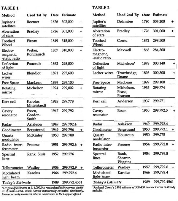
The measurement error term represents variability in the procedure's estimate, whether it be human variability in carrying out the procedure, or lack of precision in the measuring devices, etc. An example occurs in Roemer's 1676 estimate of c, which involved estimation of the diameter of the earth's orbit. Roemer inaccurately measured it, and this resulted in a low c value of 214,000 km/sec. In this case, we can eliminate this noise by substitution of the correct diameter; then Roemer's estimate is 302,000 km/sec (Froome and Essen).

Bias has at least two components. First, the procedure itself may exhibit a bias towards overestimating (or underestimating) c. Second, the experimenter may have subconsciously allowed preconceived notions of c's value to interfere with his estimate, such as knowledge of previous estimates of c or theoretical values for c at the time. Our model thus expands to:

    estimate = velocity of c + procedure bias + experimenter bias + measurement error

Consider the collection of all c estimates through time. Clearly they aren't independent, because estimates obtained from the same procedure will exhibit the same procedure bias, and estimates obtained from the same experimenter will exhibit the same experimenter bias. Instead, consider the collection consisting of one estimate, say the earliest, from each procedure. Each estimate has a distinct procedure bias value associated with it, not related to the other estimates' procedure bias values. If no experimenter appeared twice in this collection, then each estimate also has a distinct experimenter bias value. Assume the values for the distinct procedure biases are roughly independent, distributed symmetrically about zero, and expected to average to zero. Assume the same properties for the distinct experimenter biases, and for the measurement errors. Then if NH is true, the chance that any past estimate in this collection exceeds today's c estimate is 1/2 , i.e., the box model is adequate. Using this chance, the P-value is the probability that at least as many estimates exceed today's estimate as was observed.

How willing are we to make the assumptions above? Measurement errors are most likely at least roughly independent, symmetrically distributed, and expected to be zero. But the assumptions on procedure and experimenter biases imply a rather haphazard historical development of the procedures and their results. While it may be that electrical measurements are independent of optical measurements of c, the different procedures within these groups may not be. Of even more concern is experimenter bias. Cornu's (1874) estimate of 300,400 km/sec was the average of numerous toothed wheel/deflection of light experiments, weighted in what he felt was an appropriate manner. Dorsey (1944) thoroughly studied these same observations and concluded they estimated c as 299,900. One might speculate that Fizeau's (1849) toothed wheel estimate of 315,000 may have impaired Cornu's judgement of his data. In summary, one must be aware that the bias assumptions probably are, at best, only roughly true.

Test Results

Test results indicate high P-values. Table 1 lists the earliest procedure estimates data. Four out of the seven  estimates before 1901 exceed today's value. The chance of observing four or more exceedances under NH (i.e. the P-value) is 0.50. Only six out of thirteen exceedances were observed before 1951, corresponding to a P-value of 0.71. Data after 1950 could be used, but if a decreasing c has reached an asymptote recently, then indeed, modern estimates may essentially be estimating the constant 299,792.5, and so our test would lose sensitivity to departures from the NH. For completeness, using all of the data gives 8 out of 17 overestimations of c, and thus a P-value greater than 0.5. Even if we data-snoop, i.e. look at the data before deciding which of it to use (which renders the P-value meaningless), the smallest P-value obtainable is 0.06, (the chance that the first four estimates of c exceeded today's value).

Undoubtedly, procedures were improved the second time around. Bias and measurement error may have been substantially reduced. Therefore, a collection of second earliest estimates (Table 2) may indicate more departure from NH. To remove some experimenter bias, an experimenter could only appear once in our data (Michelson appears twice, the second with two other authors which seemed to be OK; this problem didn't come up in Table 1). Unfortunately for the recent creationists, the P-values are exactly the same for Table 2 as those calculated for Table 1.

The sign test is not very sensitive, but more sensitive tests (e.g., t-test, sign-rank test) require assuming identically distributed errors for each of the noise terms in our model. Undoubtedly, the variability in these noise terms is changing (probably decreasing) as new procedures are found, so this additional assumption shouldn't be made. One might weight earlier estimates more heavily because c is larger for these under AH, but how much more is not clear because increased noise in the earlier estimates suggests not weighting them as heavily as later estimates.

The recent creationists' claim of a decreasing c, even if true, can in no way be substantiated from the results of our test. The high P-values indicate the null hypothesis of a constant c as very plausible. This plausibility, it must be admitted, may just be a reflection the insensitivity of our test. Lack of numerous independent measurements from the 17th and 18th centuries prevents us from deriving any conclusions from Table 1's first four data points, curiously all over-estimations of today's c. Only by prior opinion can one really decide whether or not these points actually give evidence against a constant c. In truth, with these data, this statistician can shed no light on this debate, and recommends resolving the debate via non-statistical evidence.

REFERENCES

Freedman, Pisani, and Purves (1978), Statistics, Norton, New York.

Froome and Essen (1969), The Velocity of Light and Radio Waves, Academic Press, London.