Science in Christian Perspective

Self-Reproducing Automata and the Origin of Life

ROBERT C. NEWMAN
Biblical Theological Seminary
Interdisciplinary Biblical Research Institute
Hatfield, Pennsylvania

From: PSCF 40 (March 1988): 24-31.

In recent decades a number of scientists have been active in seeking to demonstrate that life arose from inanimate matter by purely natural processes.¹ Most of their work has consisted of studying the biochemistry of simple life forms to propose steps by which the necessary level of complexity could be reached by chemical reactions, whether of greater or lesser likelihood.

In this paper, we do not intend to examine this claim directly by a discussion of biochemistry. Instead we wish to investigate the mathematical complexity of self -reproduction. For those who propose a naturalistic origin of life, a definition of a living thing as a self-reproducing machine should be satisfactory, even if others regard such a definition as too simple. What. then, can we find out mathematically about the simplest structure that can reproduce itself? How co is such a structure? What is the likelihood that structure might have formed randomly in the available time and space our universe provides? Such questions lead us to the mathematical theory of self-reproducing automata.

Von Neumann's Self-Reproducing Automaton

A survey of the literature indicates that the first person to design a mathematically feasible machine that reproduces itself was John von Neumann (19031957). A native of Hungary, von Neumann came to the U.S. in 1930 after earning his doctorate in mathematics at the University of Budapest. In 1931 he became a professor at Princeton University, and two years later a member of the Institute for Advanced Study there. Von Neumann was unusual among mathematicians, being interested in applications of all sorts and in being able to communicate easily with scientists and engineers. During World War 11 he was active in military applications of mathematics, and later served on the U.S. Atomic Energy Commission.

Although von Neumann invented the mathematical theory of games and made important contributions to both ergodic theory and the mathematical foundations of quantum mechanics, we are here interested in his pioneering work in computers, which eventually led to his mathematical theory of self-reproducing automata. Von Neumann entered the field of computers through the problem of solving non-linear partial differential equations. Here, he came to realize that mathematics had reached a stalemate in trying to obtain general solutions to such equations, but that specific cases could be solved numerically. These solutions could then be used as a guide to theorizing about general solutions.

Since numerical solutions to such equations are quite time consuming when done by hand, von Neumann did some of the earliest work on electronic computers. He was a consultant on several early models (ENIAC, EDVAC and JONIAC), suggesting improvements in physical design and memory. He also invented the idea of using flow charts for program design, and pioneered the concept of using one language for the computer and another for the programmer. In working out a theory for automatic control of computers by internal programs, he was led to a mathematical theory of automata.

In all, von Neumann produced five works on automata: (1) "General and Logical Theory of Automata," written in 1948 and published in 1951; (2) "Theory and Organization of Complicated Automata," five lectures given in 1949; (3) "Probabilistic Logics and the Synthesis of Reliable Organisms from Unreliable Parts," 1952; (4) "Theory of Automata: Construction, Reproduction, Homogeneity," 1952-53; and, (5) The Computer and the Brain, written 1955-56 and published in 1958. Items one and three are included in volume 5 of von Neumann's collected works³; item five was published as a separate book⁴ ; items two and four, in which we are particularly interested, were published posthumously as The Theory of Self-Reproducing Automata.⁵

Though von Neumann intended to eventually design a mathematical model of reproduction that would realistically simulate a simple living organism, he only lived long enough to sketch out details for a much more abstract automaton that would make a copy of itself. This automaton was completed (with a few minor corrections) by Arthur Berks. Let us look briefly at von Neumann's automaton as a preparation for our further discussion of a much simpler automaton.

Von Neumann imagined his self-reproducing automaton as an organized collection of small automata which can be represented as individual computer chips filling a large two-dimensional plane. These chips are rectangular and linked to each of their four nearest neighbors. Each chip can be in any one of 29 different states, which include a quiescent or "turned-off " state, several "warm-up" states for converting the quiescent state into functional states, and finally several functional states which would transmit information in various directions or serve as junctions for information transmission.

Von Neumann's self-reproducing automaton consisted of imposing certain initial state-values on a set of chips at time t = 0, in such a way that this set of chips would subsequently send out a construction arm and convert a quiescent set of chips nearby into a copy of itself. This automaton was rather complex, requiring an array of some 300 x 500 chips for the memory control unit, something similar for the construction unit, and a "tail" of some 150,000 chips to store information on the details of the automaton to be built.⁶

Von Neumann's self-reproducing automaton is notable, like early computers, mainly for showing that such a machine is feasible. Its enormous complexity, however, hardly gives encouragement to those who hope that a self-reproducing machine might happen by itself.

In the years since von Neumann's proposal, various attempts have been made to simplify his automaton. E. F. Codd, for instance, was able to design an automaton in which each of the constituent computer chips needed only eight states instead of von Neumann's 29.⁷ Yet Codd's automaton was still as complex as a typical electronic computer, and thus hardly likely to happen by chance.

Von Neumann's self-reproducing automaton is notable, like early computers, mainly for showing that such a machine is feasible. Its enormous complexity, however, hardly gives encouragement to those who hope that a self-reproducing machine might happen by itself.

Recently, Christopher Langton has proposed a drastic simplification of von Neuman's automaton, following up on some ideas suggested by Codd.⁸ Langton notes that the automata of von Neumann and Codd were unnecessarily complex because each was designed to be able to make any kind of automaton (depending on the information stored in the machine's long tail). Thus, each made copies of themselves as a special case of their capabilities as universal constructors. Langton notes that nothing so complicated as this is necessary, since the living things we are trying to mimic only make copies of themselves, not of some drastically different life forms. Langton thus abandons the idea that the automaton must be able to make other kinds of automata, and seeks the simplest machine that will make only a copy of itself. In what follows, let us go into some detail in order to appreciate Langton's simple self -reproducing automaton.

Following Codd, Langton represents the array of computer chips mathematically as a two-dimensional array of numbers, one for each chip, which specify the state in which each chip is presently functioning. Zero is used to represent the chip in its quiescent state, and the numbers 1 through 7 represent the other functional states. The automaton can thus be represented mathematically as a two-dimensional matrix of numbers which change with each unit of time as the machine functions.

The state of a particular chip at time t is calculated from its own state at the previous time-step t - I as well as the states of its neighbors at t - 1. What the seven functional states of the chip actually do in the machine can be chosen by the designer as he or she selects the set of "transition rules" which govern how each state changes with time. Following Codd, Langton defines state I as an element of a datapath. State 2 is used for elements of sheath material which protect the datapath. States I and 2 work somewhat like a nerve cell, which has a central core transmitting its signal protected by a sheath to keep the signal from straying, or like an insulated electric wire, as in Figure I.

The remaining numbers, now just 3 through 7, give us five signals which can be defined to tell the automaton to carry out various functions. Typically these signals will move along a datapath of I's. The direction of movement of a signal is specified by making each signal a pair of digits, the leading digit being one of the numbers 3 through 7, the following digit a zero. Figure 2 shows a 7 signal which will move to the right one step for each unit of time.

Figure 2

Datapaths form junctions where a path splits in two, as in Figure 3.

Figure 3

When a signal approaches such a junction coming, for example, from the left, it will split into two copies of the signal, one following each of the other datapaths, as in Figure 4.

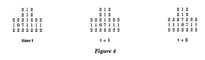
Given these features, we can design a simple device which will send a periodically repeating signal along a datapath. We simply make a closed loop with an open tail" in one corner, as in Figure 5.

Figure 5

The device shown will continually circulate its 7 - 0 signal counterclockwise around the small loop (or square, if you prefer), sending a 7 - 0 signal down the path to the right once every time the signal in the loop comes around to the junction at the lower right corner.

All this was noticed by Codd. It took the genius of Langton to observe that in this one simple device we already have the makings of a self-reproducing machine, without adding a lot of additional complexity.

Suppose the 7 - 0 signal is so defined that, when it strikes the end of a datapath, it lengthens the datapath by one unit, as in Figure 6.

Now, suppose the 4 - 0 signal is so defined that a pair of such signals striking the end of a datapath causes the path to make a lefthand corner. It turns out that we need to use another state, 3 for example, as an intermediate step in this maneuver, leaving us with just two states, 5 and 6, for anything else we want to do.

At this point, we have the machinery necessary to send a repeating signal around a loop of the proper size such that the signal can extend the loop's arm (or tail) n units, and then make the arm turn left. If we have the signal go around the loop four times, it will make the arm fold itself around into another loop, and we can design this new loop to be the same size as the original loop.

With some judicious choices for the transition rules, remembering that these rules govern how a chip changes state at the next time-step on the basis of its previous state and the state of its four neighbors, we can design the two remaining signals, 5 and 6, to arise when a signal going around the new loop collides with a signal coming from the old loop. The 5 and 6 move away from the collision area in opposite directions. The 5 disconnects the "daughter" loop from the "mother,"  and causes the mother to form a new arm at the next corner counterclockwise from the original arm, where it will then begin the process of forming another  daughter loop. The 6 makes a new arm on the daughter loop, so that it can begin to form a "grand-daughter."

Doubtless it took LanSton a lot of experimenting to find the simplest such machine that worked, but he eventually came up with a loop ten units on a side, possessing a five-unit arm and storing its construction information in a sequence of six 7 - 0 signals followed by two 4 - 0 signals. This machine, with the signals properly located at time t = 0 (as in Figure 7), will first extend its arm six units and then make a left corner. By then, the information will have cycled around the loop once and come back again, extending the arm in the new direction six units and turning left again. In 35 time units the arm turns its first corner, in 70 its second, and in 105 its third corner. The new loop closes back on itself at t = 124, separates into two loops at t = 128, sets up the mother loop to start making another daughter at t = 147, and has the first daughter in the same state as the mother originally was (t = 0) at t = 151.

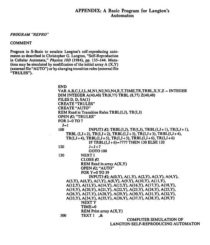
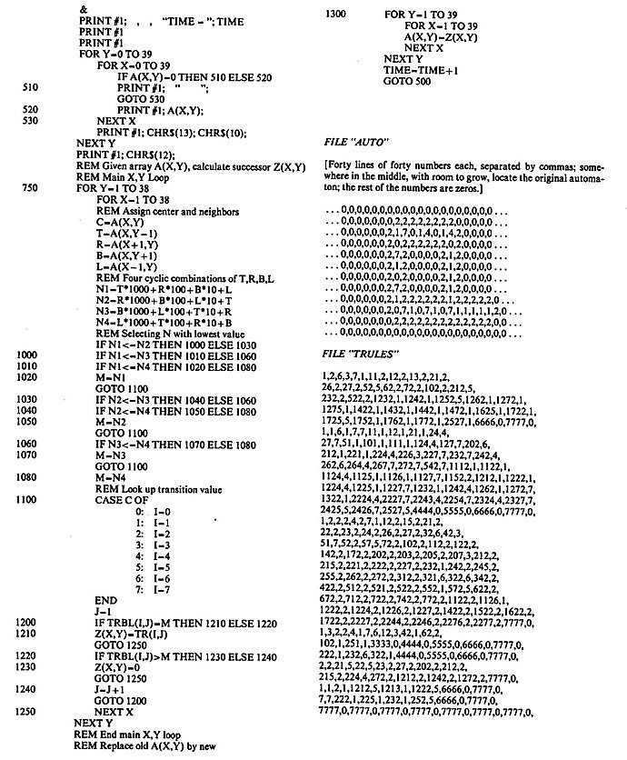
Having programmed my small personal computer in Basic to apply Langton's transition rules to his initial

loop, I can testify that it works! Due to limited memory space and a slower computer, I did not run the program past t = 153 to see the birth of third and fourth generation loops as Langton did. He provides an interesting discussion of how the loops "die" when they run out of space to make further daughters, for which 1 refer you to his original paper. A copy of my program with transition rules and a starting loop is provided in the appendix to this paper, should you wish to adapt it to your computer and experiment with it yourself. It is much more sophisticated than the public-domain computer game called "Life.

The Complexity of Langton's Automaton

So, Langton has brilliantly demonstrated that something mimicking life can be designed. Does this indicate that life arose by chance or by design? To get some feel for the answer to this question, we need to analyze the complexity of his automaton.

Clearly, Langton's device is at or near the minimum complexity for self-reproduction of any meaningful sort. The information stored in the datatrain is very small because of the loop's four-sided symmetry. Even so, to specify the particular initial state of the automaton, we must indicate the state of n chips at t - 0. Thinking of the automaton as a rectangular array of 10 by 15 chips, n = 150. Or, we can ignore chips outside the structure itself, and make n = 110. Ignoring the chips inside the "doughnut hole" of the loop, n = 94. Finally, ignoring all the zero-state chips, we can get n down to 86. For each case but the last, each chip specified could be in any one of eight states, giving 8 to the nth power combinations. For the last, each could be in any one of seven, or 7 to the nth power combinations. Table 1, in its middle column, gives the number N of possible combinations by which the chips could be specified in each case.

Thus, to produce the complexity of the initial state of the Langton automaton, we must search through some 5 x 1072 combinations for the one which works. Or, allowing for the four rotations through 90 degrees, about 1072 combinations.

However, before we attempt to estimate how likely the random formation of such a functional automaton is, we should note that most of the complexity of this device has been bidden under the rug, so to speak, in the details of the transition rules. These rules can be simplified slightly from those listed in Langton's Table 1, by eliminating all rules which put the chip in state zero and specifying instead that all rules not listed give a zero result. Even doing this, there are 190 rules producing the other seven states. To produce these randomly, we would need to search 7 to the 190th combinations, about 2 times 10 to the 160th. Combining this with the complexity of the initial state calculated above, we obtain the results N' in the righthand column of our Table 1. Again, allowing for rotations, we have about 5 x 10²³² combinations.

The number of combinations listed for the easiest case (n = 86) corresponds to the number of 276-letter words (276 = 86 + 190) one can make with a seven letter alphabet. How likely is it that such a number of combinations would be successfully searched in the history of the universe? To make such a calculation, we have to make some assumptions concerning how many objects are being searched and how rapidly.

Since it is the biochemical situation to which we will want to eventually apply our result, let us try to mimic this in a very rough way. Let us suppose that the seven letters correspond to seven common elements occurring in life chemicals, and the words correspond to strange molecules" formed of their combinations. (Please be advised that we are not doing any real chemistry here.) Let us take hydrogen as state zero and leave it out of the calculation. Let us ignore helium as unreactive and call the seven elements carbon, nitrogen, oxygen, sulfur, phosphorus, potassium and sodium. This calculation is going to be very sloppy, so let's give each element the same abundance, namely that of carbon-the most common of the seven- has a cosmic abundance about .0003 that of hydrogen.⁹

Suppose all these elements within a given volume of the universe are forming only 276-atom chains, and are forming new combinations as rapidlv as a carbon atom can move to a new chain; say, a distance of 10 Angstroms at standard temperature, 300 degrees Kelvin. (Need I point out that all these assumptions are fantastically favorable?)

Then, using Boltzmann's equation to calculate the speed of carbon atoms at 300 degrees Kelvin (8 x 10⁴ cm/sec), new chains will form at the rate of R = 8 x loll per second per chain. In the visible universe (actually the universe out to the Hubble radius), there are about 2 x 10¹² galaxies averaging 10" stars each.¹⁰ Taking our sun as an average star, it has a mass of 2 x 1033 grams. This amounts to about 4 x l0⁵⁶ grams of hydrogen within the Hubble radius. Assuming each of the seven elements being used is as common as carbon, the mass of elements reacting is about 8 x 10⁵³ grams. Using Avogadro's number and an average gram atomic weight for our elements of 24, this will give about 2 x l0⁷⁶ atoms reacting in our chains or, dividing the number of atoms per chain (276), about 7 x 1073 chains. The time to form the total number of possible combinations is then:'

time = Number of combinations N'/Number of chains x rate

time =5 x 10²³²/7 x 10⁷³) (8 x 10¹¹)

time = 10¹⁴⁷ seconds time 

3 x 10¹³⁹ years

That is a long time! We can easily convert this into a probability that this will happen in our universe, in its twenty billion year history, merely by dividing the age of the universe by the time given above. The result is:

probability = 10^-129

Conclusions

Such a probability is astronomically small. There are estimated to be only about 10⁸¹ elementary particles in the universe.¹¹uppose one of these particles were marked and we were set the task of randomly selecting this particle from all the others in the universe with no way of telling it from the others. The chance of successfully locating such a particle would be 10⁴⁸ times larger than the chance formation of a molecule with the organized complexity of the Langton automaton.

Table 1.

Unless there is some flaw in these calculations, I see only two possible responses: (1) Maybe life is designed after all. Recently, this has been the response of several formerly agnostic scientists.¹² (2) Perhaps the simplest self-replicating machine is really much simpler than the one we have analyzed. To which I respond, "Please design some such machine so that we can take your answer seriously.

Zoologist Richard Dawkins, author of The Selfish Gene, believes scientists should choose a naturalistic model for the origin of life, even if the model predicts it is very unlikely to happen. He suggests that since there may be as many as 1020 earth-like planets in the universe, and since it took about one billion years for life to show up on earth, we should admit any model in which the formation of life on a given earth-like planet has a probability of only I in 10 to the 20th.¹³ According to our calculations here, the probability of forming a simple self-replicating molecule is more than 10¹⁰⁰ less than Dawkin's threshold. It seems to me that we are looking at very strong evidence that life is designed.

REFERENCES

¹ See, e.g., Cyril Ponnamperuma, The Origins of Life (New York: Dutton, 1972); Stanley L. Miller and Leslie E. Orgel, The Origins of Life on Earth (Englewood Cliffs, NJ: Prentice-Hall, 1974); John Farley, The Spontaneous Generation Controversy from Descartes to Oparin (Baltimore: Johns Hopkins, 1977); Sidney W. Fox and Klaus D@, Molecular Evolution and the Origins of Life (New York: Marcel Dekker, 1977).

²See, e.g., Charles B. Thaxton, Walter L. Bradley and Roger L' Olsen, The Mystery of Life's Origin: Reassessing Current Theories (New York: Philosphical Library, 1984); Robert Shapiro, Origins: A Skeptic's Guide to the Creation of Life on Earth (New York: Summit Books, 1986).

³John von Neumann, Collected Works, A.W. Taub, ed. (New York: Pergamon Press, 1961-63, 6 vols.).

⁴John von Neumann, The Computer and the Brain (New Haven, CT: Yale niversity Press, 1958).

⁵John von Neumann, Theory of Self-Reproducing Automta, ed. and completed by Arthur W. Berkeley (Urbana, IL: University of Illinois Press, l966). The biographical data on von Neumann comes from this source.

⁶Theoryof Self-Reproducing Automata gives no size information for the whole machine. Berks gives 337 x 547 for the Memory Control Unit on p. 261 and notes (p. 280) that von Neumann never finished the Construction Unit. An earlier popular discussion of von Neumann's machine is given in John Kemeny, "Man Viewed as a Machine, " Scientific American 192 (April 1955):18, 58-67; reprinted in Mathematics in the Modem World (San Francisco: W.H. Freeman and Co., 1968), chap. 50. Kemeny's size estimate, 80 x 40 chips with a 150,000 chip tail, is certainly too small for the final functional version.

⁷K.  F. Codd, Cellular Automata (New York: Academic Press, 1968).

⁸ C. G. Langton, "Self-Reproduction in Cellular Automata," Phsica 10D (1984):135--144.

⁹See, e.g., the relative cosmic abundances in The McGraw-Hill Encyclopedia of Astronomy (1983), p. 108.

¹⁰Calculations based on information from Martin Harwit, Astrophysical Concepts (New York: Wiley, 1973), pp. 42,61.

¹¹Give or take a few orders of magnitude. See our number above for the total amount of hydrogen and multiply by Avogadro's number, times two to count the electrons - this is a few orders of magnitude larger if the neutrons and photons are included.

¹² See, e.g., Fred Hoyle and Chandra Wickramasinghe, Evolution (New York: Simon and Schuster, 1981); Dean H. Kenyon, in Forward to Thaxton, Bradley and Olsen, The Mystery of Life's Origin.

¹³Richard Dawkins, The Blind Watchmaker (New York: Norton, 1986), 143-146.